Day 9: Formation of Differential Correction Data and Quality Control
Lecturer: Dr. Andrew, Senior Researcher, Navigation Systems Laboratory
Date: March 2003
Introduction
Greetings, inquisitive minds! Welcome to Day 9 of our exciting course! We find ourselves in the year 2003, and today we will dive into the heart of satellite navigation to thoroughly study the process of forming differential correcting information (DCI) and the methods of controlling its highest quality. Imagine you are using a GPS navigator in your car or on a research vessel, and it determines your location with an accuracy of a few meters! Behind this technology, already changing our lives, lies a complex symphony of mathematical algorithms and fundamental laws of physics. Our goal today is to explain these principles step by step, guiding you through the labyrinth of formulas to the summit of understanding. Are you ready for new intellectual discoveries? Then let's go, onward to knowledge!
Historical Reference: How Accuracy Became Reality
Before delving into the technical details, let us take a brief historical excursion. The GPS system officially began with the launch of the first Navstar 1 satellite in 1978, starting a global navigation revolution. However, the early days of GPS were far from perfect: atmospheric delays and the drift of atomic clocks on the satellites reduced accuracy to tens of meters. In the 1980s, engineers developed Differential GPS (DGPS), significantly improving accuracy—to just a few meters. By the early 1990s, DGPS was widely used in marine navigation and geodesy. In 1995, GPS achieved full operational capability, and in 2000 the United States disabled Selective Availability (SA), making the signal more accurate for civilian users. Today, in 2003, we see how GPS and GLONASS are beginning to change the world, from marine navigation to the first automotive GPS systems!
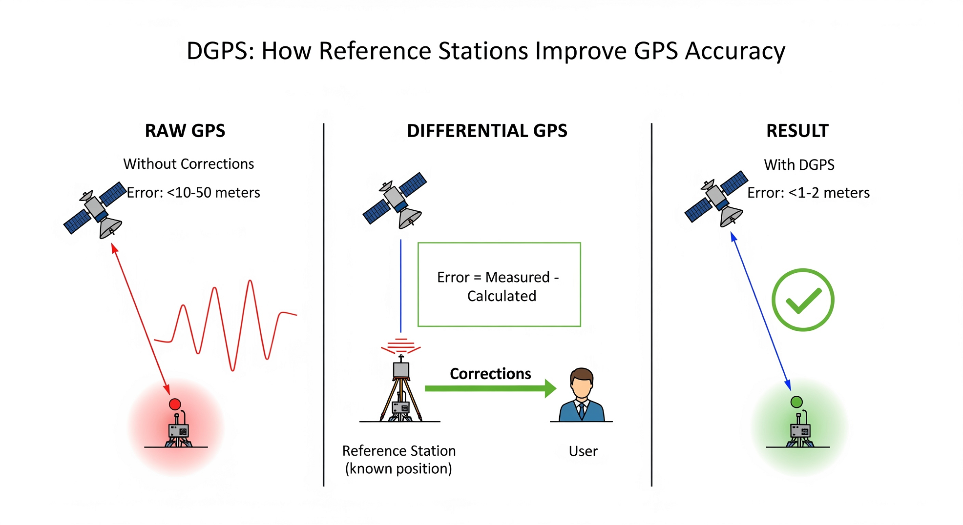
9.1. Calculating Differential Corrections in Telemetry Navigation Information
So, the starting point of our journey is the interaction between navigation space vehicles (NSV)—GPS, GLONASS, INMARSAT satellites—and receiver-navigation stations (RNS) on Earth. NSVs emit signals, and RNS units capture them. But these signals are far from ideal: the atmosphere distorts them, and even though the satellites' atomic clocks are very precise, they still have microscopic deviations. Differential corrections are our tool to say, "Enough chaos! Let's fix this navigation confusion!"
The process of computing DCI in telemetry navigation information (TNI) is akin to tuning an orchestra before a concert: a strict algorithm synchronizes all the elements to within fractions of a millisecond, ensuring the harmonious 'sound' of accurate navigation.
9.2. Forming Estimates of Differential Corrections
Imagine a coordinated team of satellites (NSV) and ground stations (RNS) working in unison. For each satellite-station pair, we calculate corrections, referencing the GPS time scale (GPST). Why GPST? Historically, it serves as the established reference, providing a single point of reference. A key factor is the signal's passage through the troposphere and ionosphere, where charged particles and water vapor act like "traffic jams," delaying radio waves and introducing errors. Here are the formulas that help us compensate for these effects:
For pseudoranges (distances measured to the satellite, including errors):
For pseudospeeds (the rate of change of distance):
Let us break down what is happening here:
- \(S^{[2]}\) — a vector of measured pseudoranges corrected for atmospheric distortions using the coefficients \(\alpha_{i,j}\). Think of these coefficients as "atmospheric glasses," allowing the signal to "see" through interference!
- \(\dot{S}^{[2]}\) — a vector of pseudospeeds, also corrected.
- \(R\) and \(\dot{R}\) — the ideal distances and speeds computed from coordinates: \(R_{i,j} = \sqrt{(x_j - X_i)^2 + (y_j - Y_i)^2 + (z_j - Z_i)^2}\).
- \(A\) — the geometry matrix describing the positioning of satellites and stations. In a real system, its dimensionality is determined by the number of NSV-RNS pairs (\(L \times L\)).
- \(K_{\text{GLONASS}}\) — a coefficient for taking into account GLONASS-specific features (1 for GLONASS, 0 for GPS), reflecting differences in time scales.
- \(\Delta \tau_i\) and \(\Delta \dot{\tau}_i\) — time and frequency corrections for clock synchronization.
These formulas are a navigation puzzle! We solve it using the least squares method, minimizing errors.
9.3. Smoothing Estimates of Differential Corrections
Having obtained the "raw" estimates, we smooth them out, taking into account the registration time \(t_{z-count}\):
where
Here, \(t_1\) is the time in seconds, which we break down into hours and a remainder, rounding with a 0.6-second step—like setting an alarm with a convenient interval! \(\frac{R_{i,j,k}}{c}\) is the signal transit time (\(c = 299,792,458 \,\text{m/s}\)).
Numerical example: Let \(\Delta S_{i,j,k} = 10 \,\text{m}\), \(\Delta \dot{S}_{i,j,k} = 0.1 \,\text{m/s}\), and \(\left(t_{z-count} - (t_i - \Delta \tau_i - \frac{R_{i,j,k}}{c})\right) = 2 \,\text{s}\). Then:
9.4. Analysis and Quality Control of Corrections
Now let's check the quality! If we have only one estimate from an RNS, we accept it with \(Health_{i,j} = 0\) and a standard deviation \(\sigma_{i,j,k}\). But if two or more estimates are available, we conduct a statistical analysis. We calculate the standard deviation:
where the weighted mean is:
For speeds, it is analogous:
Numerical example: Suppose the estimates are \(\Delta \hat{S}_{1,j,k} = 10\,\text{m}\), \(\Delta \hat{S}_{2,j,k} = 11\,\text{m}\), \(\Delta \hat{S}_{3,j,k} = 12\,\text{m}\), and \(\zeta S_{i,j,k} = 0\). Then:
The "10−10 safeguard": This coefficient in the denominator is a "lifeline." If \(\sigma S_{i,j,k,2} = 0\), then \(10^{-10}\) prevents division by zero—like a shim under a wobbly chair!
We compare \(\sigma_{\Delta \hat{S}_{j,k}}\) with the threshold \(\sigma_{\max \Delta S}\). If \(\sigma_{\Delta \hat{S}_{j,k}} < \sigma_{\max \Delta S}\), the corrections are reliable (\(Health_{j,k} = 0\), \(\zeta S_{i,j,k} = 0\)). If we detect anomalies (\(\left|\Delta \hat{S}_{i,j,k} - \Delta \bar{S}_{j,k}\right| > 2 \cdot \sigma_{\Delta \hat{S}_{j,k}}\)), we set \(\zeta S_{i,j,k} = 1\) and repeat the analysis.
9.5. Checking Acceptable Value Limits
We verify that the corrections do not exceed physical limits:
Why these values?
- 10,485.44 m: This is not an arbitrary number — it is the maximum value representable in the Pseudorange Correction (PRC) field of the international RTCM SC-104 differential-GPS message format (Type 1, scale factor 1): a 16-bit signed field with 0.32 m resolution, giving \(32{,}767 \times 0.32 = 10{,}485.44\,\text{m}\). RTCM SC-104 has been a public standard maintained by the Radio Technical Commission for Maritime Services since 1983.
- 4.064 m/s: Likewise, this is the maximum value of the corresponding 8-bit Range-Rate Correction (RRC) field at the same scale factor, with 0.032 m/s resolution: \(127 \times 0.032 = 4.064\,\frac{\text{m}}{\text{s}}\).
If the condition is not met, \(Health_{j,k} = 1\) — that satellite is marked as unhealthy.
9.6. Additional Control with a Monitoring Receiver
A monitoring receiver (MR) with known coordinates is our "golden standard." We use the Newton-Gauss method to verify the corrections. This method is not a specialized navigation technique — it combines Newton's iterative root-finding method (17th century) with Gauss's method of least squares, published in 1809 ("Theoria Motus Corporum Coelestium"), and remains the standard, openly taught approach for nonlinear position-fixing in receivers worldwide:
Newton-Gauss iterations example:
- Step 1: Initial approximation: \(\overrightarrow{\widetilde{\Theta}}_0 = [0, 0, 0, 0, 0]^T\)
- Step 2: First iteration: \(\Delta \overrightarrow{\widetilde{\Theta}}_1 = [100 \,\text{m}, 50 \,\text{m}, 200 \,\text{m}, 0.001 \,\text{s}, 0.0001 \,\text{s/s}]^T\), error: \(\sqrt{100^2 + 50^2 + 200^2} = 229.1 \,\text{m}\)
- Step 3: Second iteration: \(\Delta \overrightarrow{\widetilde{\Theta}}_2 = [10, 5, 20, 0.0001, 0.00001]^T\), error: 22.9 m
- Step 4: After 5 iterations: \(\Delta \overrightarrow{\widetilde{\Theta}}_5 = [0.005, 0.002, 0.008]^T\), error: \(\sqrt{0.005^2 + 0.002^2 + 0.008^2} \approx 0.0095 \,\text{m} < \varepsilon_{\Theta} = 0.01 \,\text{m}\). Stop! Accuracy achieved: 0.95 cm!
Lecture Conclusion
You have learned how differential corrections turn "noisy" signals into accurate coordinates, as if assembling a puzzle from thousands of measurements. In 2003, DCI was already actively used in marine navigation (for example, for precise vessel positioning), in geodesy for map creation, and in the first automotive GPS navigators from companies like Garmin and Magellan, just starting to appear in cars. These technologies pave the way to a future where satellite navigation will become an integral part of our lives.
Question to Ponder: What happens to accuracy if the ionosphere increases its influence (e.g., due to a solar flare)? What measures can be taken? Until next time in the world of science and technology!
Glossary
- Pseudorange
- The measured distance to a satellite, including errors
- Pseudospeed
- The rate of change of that pseudorange
- Relativistic effects
- Changes in time due to gravity and velocity (Einstein's theory). Atomic clocks on satellites (rubidium/cesium, stability \(10^{-13}\)) correct for these effects
- NSV
- Navigation Space Vehicles: GPS, GLONASS, INMARSAT satellites
- RNS
- Ground tracking stations (Receiver-Navigation Stations)
- \(\varepsilon_{\Theta} = 1\,\text{cm}\)
- The accuracy target for the Newton-Gauss method
- Newton-Gauss method
- An iterative method for coordinate refinement