Day 6: Introduction of Corrections (Part 2) — Troposphere and Ionosphere
Lecturer: Dr. Andrew, Senior Researcher, Navigation Systems Laboratory
Date: March 2003
1. Introduction: Why Are Corrections Needed?
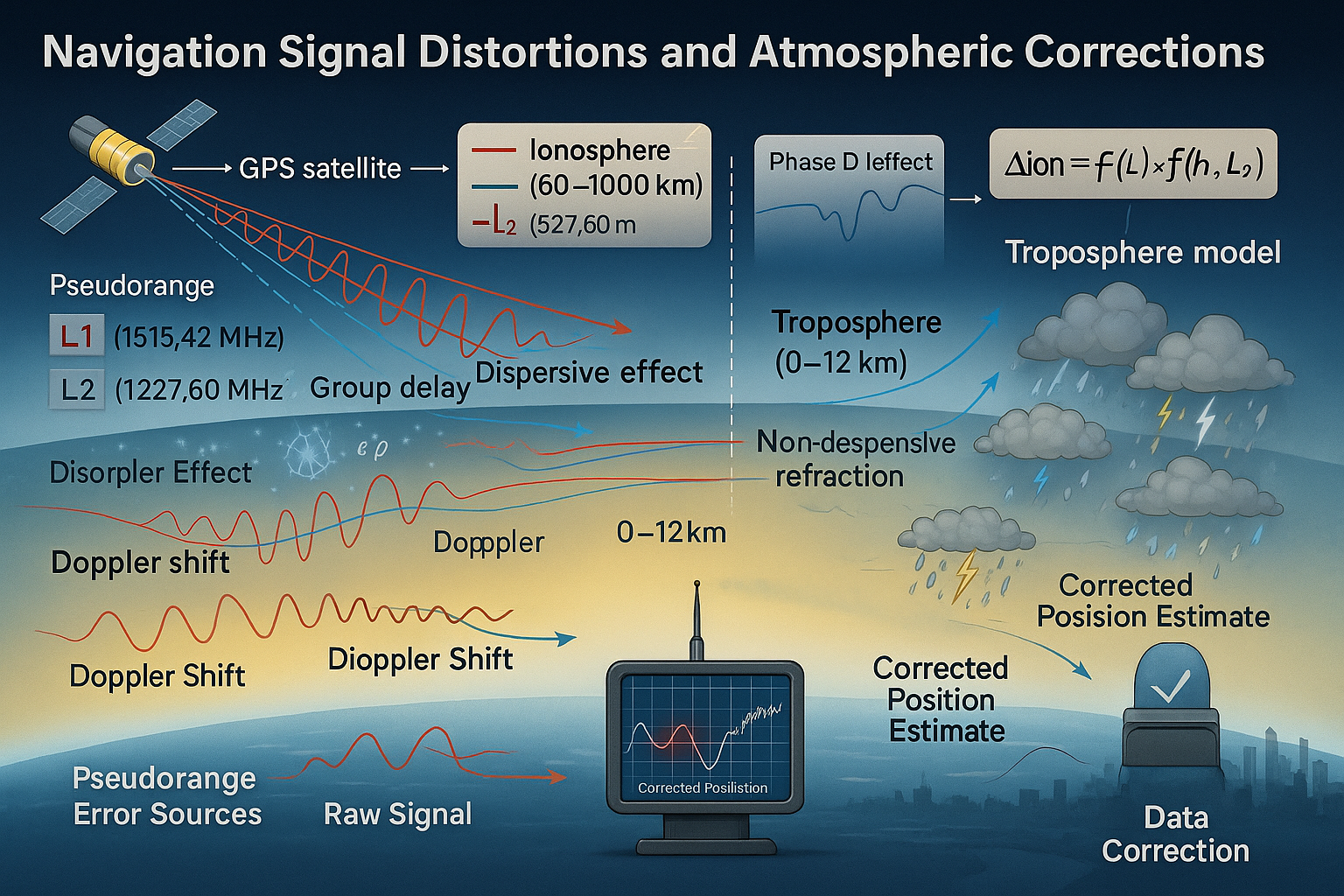
Satellite navigation operates similarly to an echo-based distance measurement. A satellite sends a radio signal, the receiver on Earth captures it, and the distance is calculated based on signal travel time. However, Earth's atmosphere acts as a multi-layered filter, slowing down and distorting the signal path.
- Troposphere (0–12 km) – a dense lower atmospheric layer where air pressure, temperature, and humidity slow down signals.
- Ionosphere (60–1000 km) – a region full of free electrons that bend and delay radio waves.
If uncorrected, these effects can introduce position errors up to tens of meters, making navigation as unreliable as a blurred city map. Corrections help eliminate these distortions, ensuring precise positioning.
2. Glossary of Key Terms
- Pseudorange
- Measured distance to a satellite, including signal delay errors.
- Pseudovelocity
- Estimated velocity of the receiver based on signal frequency shift.
- Doppler Shift
- Frequency change due to relative motion between the receiver and satellite.
- Elevation Angle
- Angle between the satellite and the observer's local horizon.
- Group Delay
- Frequency-dependent delay of radio waves in the ionosphere.
- Free Electrons
- Charged particles in the ionosphere affecting signal speed.
3. What Are Pseudorange and Pseudovelocity?
Pseudorange \( \tilde{\rho} \)
Pseudorange is the calculated distance based on signal travel time:
where:
- \( c = 299,792,458 \) m/s – speed of light
- \( \Delta t \) – signal travel time
Why "pseudo"? The time \( \Delta t \) includes errors from:
- Tropospheric and ionospheric delays
- Clock synchronization issues
- Receiver noise
Example: If the signal delay is \( 0.0001 \) s:
After applying corrections, the actual distance might be 29.5 km.
4. Tropospheric Correction Model
Tropospheric delay correction for the dry component is computed using the Saastamoinen model:
where:
- \( T \) – temperature (Kelvin)
- \( P \) – pressure (hPa)
- \( \varepsilon \) – satellite elevation angle
- \( a, b \) – empirical coefficients
5. The Saastamoinen Model
The Saastamoinen model is widely used in satellite navigation for estimating tropospheric delay. Developed by Finnish scientist Jorma Saastamoinen and published in 1972, it is a publicly documented model that has become a standard for atmospheric corrections in GNSS systems worldwide.
Principles of the Model
Physical Meaning: The model accounts for signal deceleration due to air pressure, temperature, and humidity. These factors are included in the formula as key variables.
Mathematical Basis:
The Saastamoinen model improves GNSS accuracy, making it a crucial tool for high-precision navigation.
6. Ionospheric Corrections
The ionosphere affects radio signals differently at different frequencies. For dual-frequency receivers, we can calculate ionospheric corrections directly:
where:
- \( S_{L1}^{j}, S_{L2}^{j} \) – pseudoranges on L1 and L2 frequencies
- \( f_{L1} = 1575.42 \) MHz – L1 frequency
- \( f_{L2} = 1227.60 \) MHz – L2 frequency
For pseudovelocity corrections:
7. Combined Corrections Application
The final corrected pseudorange and pseudovelocity are calculated as:
where:
- \( S_{i,j,k,2} \) – filtered pseudorange from Day 4
- \( \Delta_{trop}^{j} \) – tropospheric correction
- \( \Delta_{ion}^{j} \) – ionospheric correction
8. Practical Example
Let's calculate corrections for a satellite at 30° elevation:
Given:
- Temperature: T = 288 K (15°C)
- Pressure: P = 1013 hPa
- Elevation angle: ε = 30°
- Dual-frequency pseudoranges: SL1 = 20,000,000 m, SL2 = 20,000,010 m
Tropospheric correction (simplified):
Ionospheric correction:
9. Summary
Atmospheric corrections are essential for accurate GNSS positioning:
- Tropospheric corrections depend on weather conditions and satellite elevation
- Ionospheric corrections depend on solar activity and can be calculated using dual-frequency measurements
- Without these corrections, positioning errors can exceed 20-30 meters
- With proper corrections, centimeter-level accuracy is achievable
Tomorrow, we'll explore how to analyze the quality and integrity of these corrected measurements.