Day 3: Sequence of Measurement Data Processing

Lecturer: Dr. Andrew, Senior Researcher, Navigation Systems Laboratory

Date: March 2003

Introduction to the Journey

Welcome to the third day of our adventure! Today, the students arrived on time, and Andrew started a brief lecture to immerse us in the essence of the Coordinate-Time and Navigation Support System (SKNOU). We will explore the sequence of measurement data processing, which reflects the stages described in the preliminary data processing. Here, raw signals are transformed into valuable navigation data. Let's break down this process step by step, paying close attention to the formulas that form the foundation of these transformations.

Journey of Data: Extended Version with Formulas

DATA-PIZZA 2.0

Infinite Kitchen Loop — Algorithmic Art

🏠 0. RECIPE INITIALIZATION

                            recipe_params ← LOAD_DEFAULT_RECIPE()
                        

Technical Mapping:

INIT_DEFAULT_FILTER_PARAMS

WHILE oven_is_hot (system_is_running)

∞

🥘 INGREDIENT ACQUISITION

                                ingredients ← GATHER FROM Pantry()
                            

Raw Data → GNSS Frames → NRS Buffer

Technical Mapping:

ACQUIRE raw GNSS frames FROM each NRS

🧽 PREP & SANITIZE

PREP ingredients

SCALE ingredients

DISCARD spoiled_items

Technical Mapping:

UNPACK frames

DECODE DI → integers, CONVERT to SI units

DETECT & REMOVE outliers

🍞 DOUGH SMOOTHING

                                dough ← MIX ingredients USING recipe_params
                            

ANALYZE dough_texture()

REST dough UNTIL synced_clock()

STORE dough IN WalkInFridge

Technical Mapping:

FILTER data USING current params

RUN statistical_analysis

TIME_ALIGN DI

PUSH filtered_data TO RPKNP_DB

🧂 FLAVOR CORRECTIONS

                                kitchen_context ← FETCH FROM WalkInFridge
                            

SEASON sauce USING kitchen_context

Technical Mapping:

PULL geo_context / models FROM RPKNP_DB

APPLY measurement_corrections

🔍 INTEGRITY CHECK

                                integrity_flag ← VERIFY oven_temp_and_hygiene()
                            

Technical Mapping:

MONITOR navigation-field integrity

🍕 BAKE & BUILD DCI

                                pizza ← BAKE dough WITH integrity_flag
                            

Technical Mapping:

BUILD optimal_DCI WITH integrity_flag

✅ QC & DELIVERY

                                IF INSPECT pizza == PASS
                            

                                  SLICE_AND_BOX pizza FOR Delivery
                            

                                  recipe_params ← SEND_SLICE_TO_CCS_GET_TUNING()
                            

                                  ARCHIVE {dough, pizza, logs} IN WalkInFridge
                            

                                ELSE
                            

                                  LOG "🍕 Burnt pie – discarded"
                            

Technical Mapping:

VALIDATE dci_packet

ENCODE DCI FOR end-user distribution

FORWARD MI/DI TO CCS & GET new filter params

STORE {filtered_data, dci_packet, logs} IN RPKNP_DB

Pizza Action	Engineering Step	Purpose
GATHER FROM Pantry	Acquire raw GNSS frames from NRS	Obtain raw measurement data
PREP / SCALE	Unpack frames, decode DI, convert to SI	Convert data to physical units
DISCARD spoiled items	Detect & remove outliers	Remove anomalous measurements
MIX / REST	Filter, stats, time-align	Clean & synchronize data stream
SEASON sauce	Apply measurement corrections	Compensate ionosphere, troposphere, etc.
VERIFY oven…	Navigation-field integrity monitoring	Ensure navigation-field integrity
BAKE	Generate optimal DCI	Form differential-correction packet
SLICE_AND_BOX	Encode DCI for end users	Prepare RTCM messages
SEND_SLICE_TO_CCS	Forward MI/DI to CCS & receive new params	Close feedback loop
ARCHIVE … IN WalkInFridge	Store data & logs in RPKNP_DB	Historical database for audit & analysis

GNSS data gathering from satellite pantry

Scene 1 — Gather from Pantry

The chef gathers raw GNSS data represented by glowing cubes falling from satellites.

1. Receiving Raw Data: The Heroes' First Steps

The journey begins with the reception of raw data from satellite signals. These signals, encoded with navigation messages, arrive as binary streams. The first task is to verify their integrity using control sums, such as CRC (Cyclic Redundancy Check) or XOR-based checks, as described in the preliminary processing stage. This ensures no corruption occurred during transmission.

The pseudorange, a key metric, is introduced here with the formula:

\[ \rho = c \cdot (t_{\text{recv}} - t_{\text{send}}) \]

where:

\(c\) is the speed of light (299,792,458 m/s)
\(t_{\text{recv}}\) is the reception time
\(t_{\text{send}}\) is the transmission time

This formula sets the stage for later calculations, though its full application comes in subsequent steps.

2. Preliminary Data Processing: Converting to Physical Units

Next, the verified raw data is converted into physical units. This involves applying scale factors to transform digital counts into meaningful measurements like distances or velocities.

For example, a scale factor \(k\) multiplies the raw data \(D_{\text{raw}}\) to yield a physical value \(D_{\text{phys}}\):

\[ D_{\text{phys}} = k \cdot D_{\text{raw}} \]

Table 5.1 from the preliminary processing details these factors for parameters like azimuth, Doppler shift, and time. This step ensures compatibility with navigation algorithms, though synchronization of time scales (e.g., GPS vs. GLONASS) is noted here as a future consideration.

3. Kepler's Algorithm and Satellite Coordinates: Ephemerides

With physical units in hand, we calculate satellite coordinates using ephemeris data.

GPS Satellite Position Calculation

For GPS, the Keplerian orbit model is employed. The process starts with the mean anomaly \(M\), which evolves to the eccentric anomaly \(E\) via the Kepler equation:

\[ M = E - e \sin(E) \]

where \(e\) is the eccentricity. This is solved iteratively, leading to the true anomaly and finally the position \((X, Y, Z)\) in the Earth-Centered Earth-Fixed (ECEF) frame.

GLONASS Satellite Position Calculation

For GLONASS, numerical integration (e.g., Runge-Kutta method) adjusts for its non-Keplerian orbit, as detailed in the preliminary processing. These calculations are critical for positioning.

4. Corrections: Earth Rotation (Sagnac Effect)

Corrections refine our data. The Sagnac effect, caused by Earth's rotation, adjusts the pseudorange. The correction \(\Delta_{\omega}\) is computed as:

\[ \Delta_{\omega} = \frac{2 \omega_E R_E^2}{c} \cdot \sin(\phi) \]

where:

\(\omega_E\) is Earth's angular velocity (7.2921151467 × 10⁻⁵ rad/s)
\(R_E\) is the Earth's radius (6,371,000 m)
\(c\) is the speed of light
\(\phi\) is the latitude

This aligns with the preliminary processing's focus on rotation corrections, though ionospheric and tropospheric effects are noted as UNIX-specific enhancements for future implementation.

5. Quality Analysis and Integrity Checks

Quality checks ensure data reliability. While the preliminary processing focuses on control sums (Section 5.1), additional metrics like PDOP (Position Dilution of Precision) could enhance integrity. However, these are not detailed yet and serve only as a conceptual note tied to the pseudorange formula \(\rho\). Further development is needed beyond the current scope.

6. Forming Differential Corrections (DC) and Data Output

Finally, differential corrections are formed using pseudoranges. The code pseudorange \(S_{C/A}\) is calculated as:

\[ S_{C/A} = \rho + c \cdot (dt_{\text{recv}} - dt_{\text{send}}) \]

where \(dt_{\text{recv}}\) and \(dt_{\text{send}}\) are receiver and satellite clock offsets. These values, derived in the preliminary processing, enable output in formats like raw data archives, ready for navigation use.

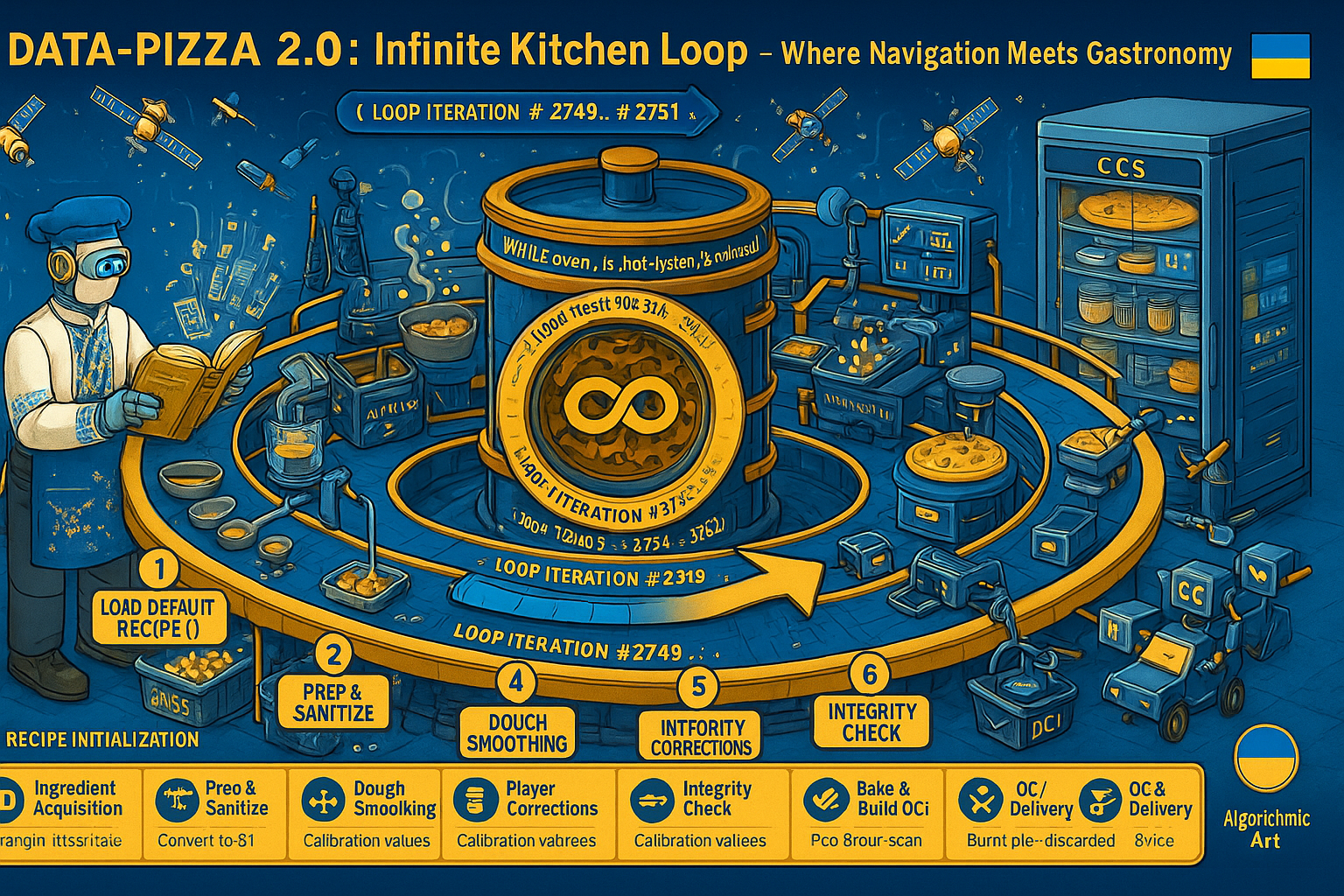
7. Humorous Epilogue: Data-Pizza 2.0

Imagine our data as a pizza! The crust is the raw data, topped with sauce (physical units), cheese (satellite coordinates), and extra toppings (corrections). Delivered hot, it's ready to navigate—UNIX style, of course!

A humorous infographic called 'DATA-PIZZA' illustrating the step-by-step process of GNSS data processing from raw signals to a final navigation solution — The Data-Pizza: From raw ingredients to navigation feast!

8. Summary

The key steps in measurement data processing:

Receive and verify raw data with control sums
Convert to physical units using scale factors
Calculate satellite positions with Kepler or numerical methods
Apply Sagnac corrections to refine pseudoranges
Form differential corrections for output

Each step builds upon the previous, transforming raw satellite signals into precise navigation solutions. The beauty lies not just in the mathematics, but in the systematic approach that ensures reliability and accuracy.

^ Back to top