Day 2: Control and Correction Station
Lecturer: Dr. Andrew, Senior Researcher, Navigation Systems Laboratory
Date: March 2003
Introduction: A Look into the Heart of Navigation
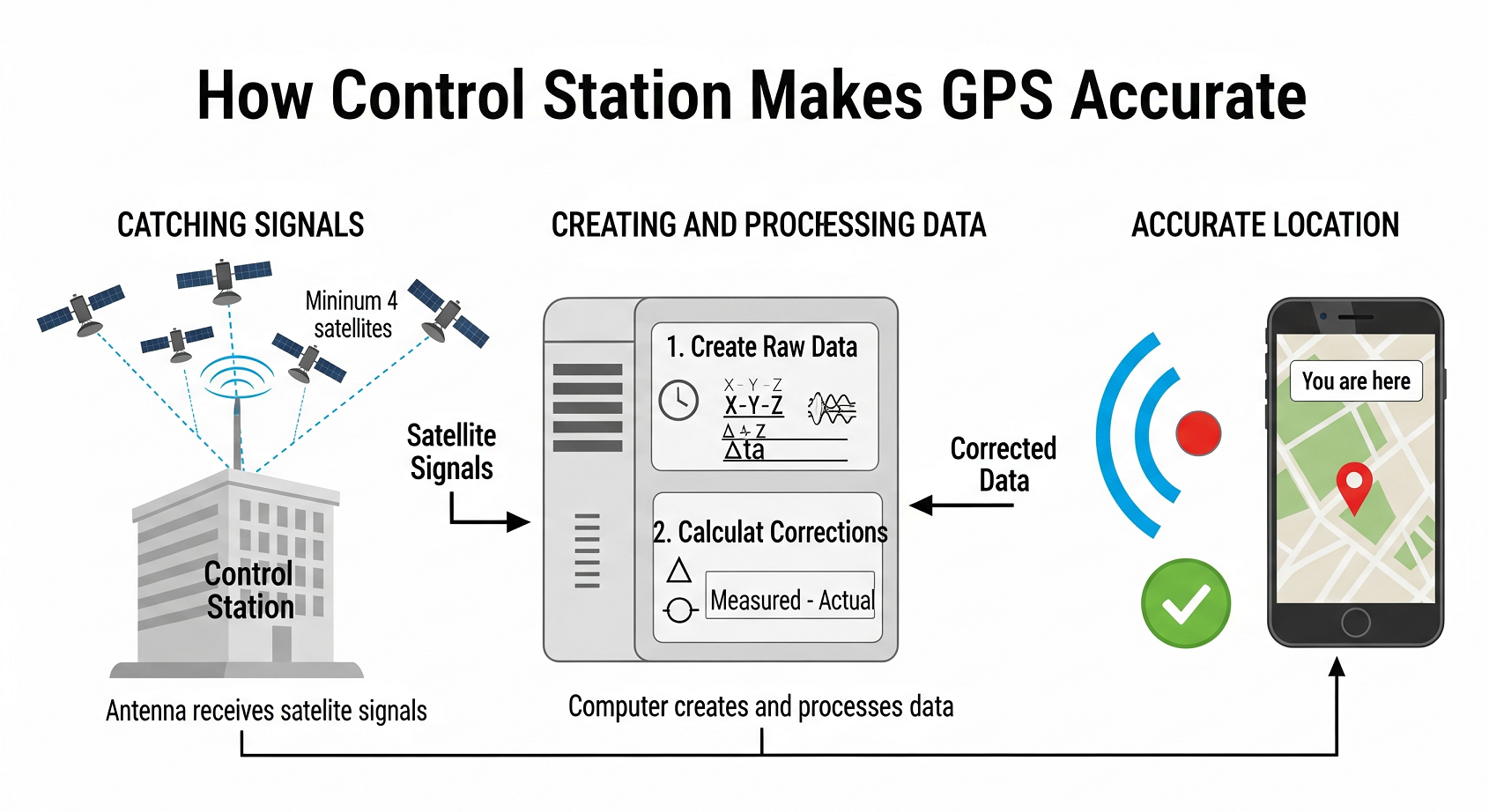
Day two of the practice began with excitement. Andrew led the students into the laboratory, where server racks hummed, and the air was filled with the spirit of technology. This was the Control and Correction Station (CCS)—not just a room with equipment, but a true control center for satellite navigation accuracy.
"This is the heart of the SKNOU system," Andrew said proudly, gesturing to the equipment. "Here, signals from GPS and GLONASS satellites are transformed into data that help us not get lost in this vast world. How does it work? It's both simple and complex. The CCS has three main heroes:"
- Roof-mounted receivers — they capture satellite signals like ears tuned to a cosmic wave.
- Computing center — the brain of the station, analyzing data and calculating corrections.
- Transmitters — the voice, sending correction signals to those who need them.
The students froze, watching the blinking lights. It felt like a journey into the future—and it was just beginning.
A Simple Explanation: What is Input Data and Why is it Needed?
Imagine: you're walking through an unfamiliar city with a trusty companion—a GPS navigator on your smartphone. It whispers: "Turn left," "You're almost there." But think: how does it know where you are? The answer lies in invisible threads connecting Earth and space—in data we call Input Data. This is the fuel without which the navigator turns into a useless piece of plastic. Let's figure out where it comes from and why it's so important.
Two Main Categories of Data
Input data is like ingredients for a delicious dish. It can be divided into two groups:
- "Raw data" — fresh, unprocessed, straight from the "cosmic garden." They are collected by receivers Z18 and GG24, which, like sensitive radio stations, catch satellite signals.
- Algorithm configuration parameters — the recipe, instructions for the program: "Add a pinch of this, mix with that." They help turn signal chaos into precise coordinates.
What's Hidden in "Raw Data"?
Raw data is a whole set of tools, like a chef's arsenal:
- Measurement data — distances to satellites, angles of visibility, small details as if measured by a cosmic ruler.
- Location data — your coordinates, like a point on a map: "You're here, at the intersection."
- GPS ephemeris — the schedule of GPS satellites, where and when they will be, like a train timetable.
- GLONASS ephemeris — the same for Russian satellites.
- GPS almanac — a general map of all GPS satellites' positions.
- GLONASS almanac — a similar map for GLONASS.
Interestingly, the Z18 and GG24 receivers "hear" measurement data differently—like two chefs using different spices—but the rest of the data is the same. All this is neatly packed into tables numbered 2.1 to 2.7. Let's take a look inside!
Revisiting Input Data: Reinforcement Through Repetition
Andrew noticed the students were thoughtful and decided to reinforce the material.
"Let's go over it one more time, just to be sure," he smiled. "Imagine you're in an unfamiliar city with only a navigator to guide you. It knows everything: where you are, where to go, how to avoid traffic. But without Input Data, it's nothing. These are data from satellites orbiting above us. They are the key to your path."
Two Categories of Data (Reinforced)
"Input data is divided into two parts," Andrew continued. "Raw data is what the Z18 and GG24 receivers catch directly from space. And configuration parameters are instructions for the program to 'cook' everything correctly."
Raw Data: Details (Repeated)
"Raw data consists of six types of information," Andrew continued:
- Measurements — distances, angles, etc.
- Location — your coordinates.
- GPS ephemeris — GPS satellite schedules.
- GLONASS ephemeris — GLONASS schedules.
- GPS almanac — general GPS satellite map.
- GLONASS almanac — general GLONASS map.
"Z18 and GG24 differ in measurements, but the rest is common. It's all in tables 2.1–2.7. Got it? Great, let's move on!"
Table 2.1: Data Structure of Measurements for the Z18 Receiver
The Z18 receiver is a real space detective. It "listens" to satellites and collects a mountain of data:
| Parameter | Size (bytes) | Description |
|---|---|---|
| ID number | 2 | Unique code updated every 50ms, reset every 30 minutes |
| Remaining structures | 1 | Number of data pieces to send in one cycle |
| Satellite number | 1 | 1-56: whose signal is caught (0 if data is scarce) |
| Elevation angle | 1 | Angle in degrees |
| Azimuth angle | 1 | Direction in double degrees |
| Channel number | 1 | Which of the 18 channels is working |
Key measurements include:
- C/A code data block (1 byte, 29 bytes inside): A structured navigation-code data block received from the satellite.
- Warning flag (1 byte): Alarm signal if something's wrong—each bit like a separate bell.
- Goodbad flag (1 byte): Data quality: 0—nothing, 22 or 23—there is data, but with caveats.
- Polarity_know (1 byte): 0—satellite just caught, 5—signal understood.
- Signal-to-noise ratio (1 byte): How loudly the satellite "shouts" above the noise.
- Carrier phase (8 bytes): How many signal waves have passed, if the function is active.
- Raw_range (8 bytes): Distance to the satellite in seconds—difference between emission and reception. Differs by 11 seconds for GPS and GLONASS.
- Doppler (4 bytes): Frequency change rate in 10,000 Hz.
- Smoothing (4 bytes): Refinement for accuracy.
- XOR control (1 byte): Check if everything is correct.
Total: 95 bytes. It's like a suitcase full of cosmic treasures!
Table 2.2: What Does the GG24 Receiver Catch?
GG24 is Z18's brother but with character. The main differences:
- Channel number (1–24): GG24 has 24 channels—more opportunities!
- Warning flag: Its own alarm signals, slightly different.
- Goodbad flag: Up to 24—data is useful.
- 37 bytes for C/A — a bit more codes.
Total: ~70–80 bytes. GG24 is another view of the same stars.
Table 2.3: Where Are We? (Location Data)
This table is like a "You are here" mark on a map:
| Parameter | Size (bytes) | Description |
|---|---|---|
| Reception time | 4 | When signal was caught (milliseconds GPS/GLONASS) |
| Place name | 4 | Note like "Laboratory" |
| Coordinates X, Y, Z | 8 each | Where the antenna is (meters) |
| Clock offset, velocities, drift | 4 each | How clock and antenna move |
| PDOP | 2 | Positioning accuracy (×100) |
Total: 56 bytes. This is your address in the vast world!
Tables 2.4–2.7: Satellite Schedules and Maps
- Tables 2.4 and 2.5: Ephemerides — The schedule of each satellite: weeks, seconds, coordinates, velocities, corrections. All in fields from 2 to 8 bytes. Like a ticket for a space train!
- Tables 2.6 and 2.7: Almanacs — The general map: satellite numbers, frequencies, their "health" (0 or 1), orbits, checks. It's like a city plan for satellites.
Algorithm Settings: The Recipe for Accuracy
Configuration parameters are instructions for the program: how to process the data so everything matches. They are described in sections 5–10. Without them, it's like cooking without a recipe.
Student Question: Why a Dual-Frequency Receiver?
"Why is a dual-frequency receiver needed? It's expensive!" a student asked, looking at Andrew.
He smiled: "Great question! Let me explain."
Answer: Why a Dual-Frequency Receiver is Essential
A dual-frequency receiver is like super glasses for navigation. Here's why:
-
The Ionosphere Interferes
The ionosphere—a layer of charged particles—distorts signals. Lower frequencies are delayed more. Signals L1 (1575.42 MHz) and L2 (1227.60 MHz) suffer differently. -
Single-Frequency Receiver
It catches only L1 and guesses the delay using models (e.g., Klobuchar). Accuracy? Not always ideal. -
Dual-Frequency Receiver
It catches L1 and L2, compares them, and calculates the delay precisely. The formula is simple:
\[ \Delta_{\text{iono}} = \frac{f_1^2 - f_2^2}{f_2^2} (\rho_1 - \rho_2) \]where \( f_1, f_2 \) are frequencies, \( \rho_1, \rho_2 \) are distances. This removes ionospheric distortions.
Conclusion: One receiver is single-frequency, the other is dual-frequency. The latter is more accurate because it conquers the ionosphere!
Andrew Simplifies Further
Andrew noticed the students were quiet and decided to add simplicity:
"Imagine: a single-frequency receiver is like listening to the radio with interference. A dual-frequency one is like pure sound in headphones. It removes ionospheric noise, and you know exactly where you are. Cool, right?"
Inspiring Finale: A Journey into the World of Navigation
Imagine: you're standing on the edge of a cliff, wind in your hair, and before you is an endless world. You open the map on your smartphone—and bam!—the "You are here" point with meter accuracy. Magic? No, it's satellite navigation, and its heart is input data.
How Does It Work?
Become an engineer for a minute:
- Receivers catch signals.
- Measure distances and angles.
- Ephemerides clarify where satellites are.
- Two frequencies defeat the ionosphere.
- You see precise coordinates.
It's not just technology—it's a dance of science and fantasy!
Why Is This Inspiring?
Satellite navigation is a bridge between us and the stars. Every time you look at a map, remember: behind each "You are here" point is the work of minds, and you can be one of them. Aircraft land safely, ships navigate, surveyors measure land, and rescue teams find their way — all thanks to these data. It's your chance to shape the future!
Conclusion: Practice Diary, Day 2
Thus passed the second day. The students saw how the CCS comes to life, learned about Input Data and dual-frequency receivers conquering the ionosphere. Andrew explained everything with fire in his eyes: satellite navigation is not just science, but a chance to touch greatness. And who knows, maybe one of them will soon create a new technology that will lead us to the stars?
If anyone snoozed through the lecture for reasons beyond their control (it happens!), don't worry. All the detailed data and structures presented in the tables are available for you to review at your own pace. Learn how to use them effectively, and you'll be able to work with this material like an expert!
Digital Polygraph application link: The labor-intensity calculator is available through the Labor Intensity Calculator.