1. PURPOSE AND SCOPE OF APPLICATION

The Remote Concentrator Software is intended to ensure the operation of the Remote Concentrator (RC) as part of the "Collection" system, functioning as a node in a computer network.

The main functions of such a node include:

1. Exchange of information via communication lines with other network nodes, including transit data routing functions;
2. Exchange of information via communication lines with subscribers (users) who are not nodes in the network;
3. Transmission of data received from non-network subscribers to network nodes and vice versa;
4. Storage of information received from both network and non-network subscribers.

Thus, the primary purpose of the Remote Concentrator Software is to establish an information interface between networked and non-networked subscribers. In cases where information delivery is not possible (e.g., due to communication line failure), the software ensures data storage in the form of files. These files are delivered later, after restoration of normal data transmission functionality. Within the "Collection" system, information from measurement systems (non-network subscribers) must be transferred through the Remote Concentrator to the data collection and processing center, and control information from the center must be delivered back to the measurement systems via the Remote Concentrator.

2. TECHNICAL CHARACTERISTICS

2.1. Problem Statement for Remote Concentrator Software Development

The Remote Concentrator Software is an integral part of the overall software of the "Collection" system. It cannot be considered separately from the core tasks solved by the system as a whole.

The primary task is to create an integrated hardware and software environment that includes all users of the "Collection" system and is designed for data collection and processing.

To build such an environment, the following common principles (requirements) must be applied for all users:

• A unified data transmission environment;
• Uniform principles of data organization and access.

In the Remote Concentrator, these principles are implemented by using the same operating system and network package as in the computer systems of the data collection center.

In addition to general requirements, the Remote Concentrator must fulfill the following specific requirements derived from the Statement of Requirements (SOR) and Specific Technical Assignment (STA):

• Data exchange with a specified set of measurement tools in accordance with defined interface and connector agreements;
• Reliable execution of functional tasks with the required level of automation;
• Adequate performance (throughput capacity).

The first requirement is met by developing RC software that supports communication protocols with currently existing measurement systems. Such systems include the "Vega-N", "Vega-K", "Vega-T", and "Kama-A" types. Connecting new measurement systems to the Remote Concentrator requires developing new exchange programs without modifying the core software.

Fulfilling the second requirement, from the software perspective, means the RC should respond consistently and adequately to exceptional situations occurring during data exchange, and be capable of resolving such situations with minimal human (operator) intervention.

Meeting the third requirement assumes high performance of the computing hardware included in the RC.

The full impact of the software on meeting the RC’s performance requirements can be assessed during the development of operational programs.

According to the SOR/STA, the RC must ensure the following performance characteristics:

• Simultaneous data exchange with measurement systems at speeds up to 9600 bps;
• Data exchange with the collection center, including real-time transfer, at speeds up to 9600 bps.

2.1.1. Hardware Composition

Two types of Remote Concentrators (RC) have been defined based on their functional capabilities (see Figure 2.1) and deployment location.

a)

b)

Figure 2.1

The Remote Concentrator (RC), see Figure 2.1(a), is installed at Measuring Points (MPs) and is designed for data exchange with Measuring Systems (MS) and the Information Collection and Processing Center (ICPC).

The RC (NI525.01), see Figure 2.1(b), is installed at the ICPC and can perform the following functions:

1. Network server for the collection center;
2. RC of the collection center with functions and software similar to NI525.

Currently, functions 1 and 2 of the NI525.01 are mutually exclusive. In the future, they are expected to be integrated.

The network server is intended to collect data from RCs located at Measuring Points. The shared part of the software for the network server and NI525 includes programs that support the generation, loading, and operation of the Synchronization Processor (SP) software.

The PC that is part of the RC has 2–4 MB of RAM and 80–120 MB of disk storage. The multiplexer included in the RC provides interfacing between the PC and the SP via an RS232 asynchronous interface line.

The functions of the SP include:

• Electrical and logical interfacing between the MS outputs and the PC input;
• Asynchronous-to-synchronous data conversion to interface the asynchronous output of the PC with the synchronous input of the data transmission equipment.

The structure of the SP is shown in Figure 2.2:

Figure 2.2

2.1.2. Data Flows Through the Remote Concentrator

To determine the functionality of the RC software, it is necessary to analyze the data flows passing through the RC. These flows are illustrated in Figure 2.3.

Figure 2.3

Flow 1 represents a stream of “task” information sent from the center to the measuring systems (MS).

Flow 2 indicates the transit transmission of measurement data from the measuring systems to the center.

Flow 3 represents data flowing from the MS to the center with both transit transmission and simultaneous recording to disk. This approach helps preserve the data in case of unstable connections with the center during a session.

Flow 4 is used to transmit data from the MS to the RC when the communication line with the center is damaged. This data is stored on disk and transmitted later upon request from the center (i.e., when the connection is restored).

Flow 5 addresses the case where the MS cannot receive data from the RC due to, for example, the absence of reception software. In such cases, the task from the center may be output to an external device (e.g., printer) for manual delivery to the MS.

Flow 6 is intended for transferring accumulated data from the RC to the center after the measurement session.

Currently, the RC software focuses on implementing the feasible flows — i.e., flows 2 through 6. Flow 1, if needed, can be supported by adding a separate program without modifying the main RC software.

2.1.3. Choice of Operating System

As noted earlier, the choice of operating system for the RC is primarily driven by the goal of creating an integrated information collection and processing environment at the central facility. UNIX was selected as the base operating system for this environment.

The key advantages of the UNIX OS include:

• Multitasking;
• Portability of the OS;
• Multi-user mode;
• Strong protection against unauthorized access;
• Support for structured programming languages;
• Advanced debugging tools;
• Powerful graphical dialog tools;
• Availability of network software packages;
• Compatibility with MS-DOS commands and files;
• Absence of viruses.

2.1.4. Choice of Network Environment

The need to build an integrated system for collecting and processing measurement data necessitated the use of a unified communication environment for both remote elements of the "Collection" system and the central data processing computers.

This requirement is met through the use of the TCP/IP network package implemented within the UNIX system.

This network software supports both distributed and local networks.

The main capabilities of the network package include:

• File exchange between network nodes;
• Access to remote files from terminals and user applications;
• Inter-process communication between processes on different nodes, allowing them to exchange data;
• Inter-terminal communication;
• And more.

3. STRUCTURE AND COMPOSITION OF REMOTE CONCENTRATOR SOFTWARE

The Remote Concentrator (RC) software, as part of the "Collection" system, consists of two main components:

• System software (operating system, compilers, drivers, etc.);
• Application software (RC-specific programs that implement the functions described in Section 1).

The composition and structure of the RC software are schematically shown in Figure 3.1.

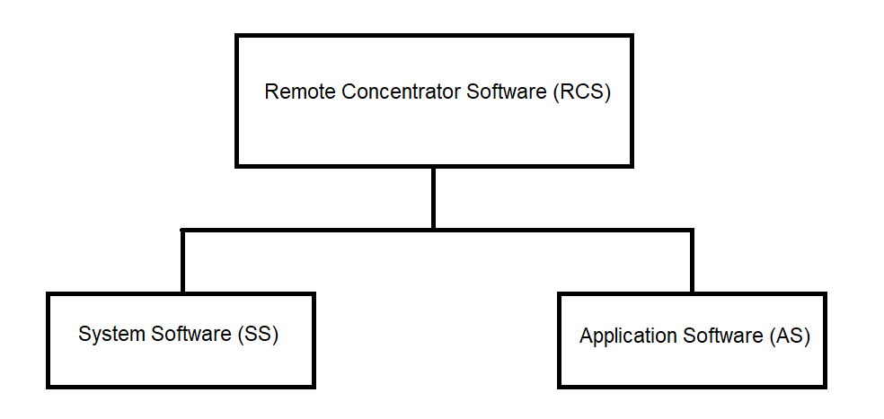
Figure 3.1

3.1. System Software of the Remote Concentrator

The system software of the Remote Concentrator (RC) consists of the following components:

• System software of the PC;
• System software of the Synchronization Processor (SP).

The structure of the RC system software is shown in Figure 3.2.

3.1.1. PC System Software

The PC system software is a set of software tools responsible for managing the PC hardware resources and coordinating the interaction between application processes and the RC hardware modules.

The PC system software includes:

• Standard PC software;
• Device drivers;
• Network software.

The standard PC software includes the UNIX operating system, which performs the following functions:

• Memory management;
• Input/output management;
• File system management;
• Process interaction control;
• Process scheduling and dispatching;
• Protection against unauthorized access;
• Resource usage accounting;
• Command language processing.

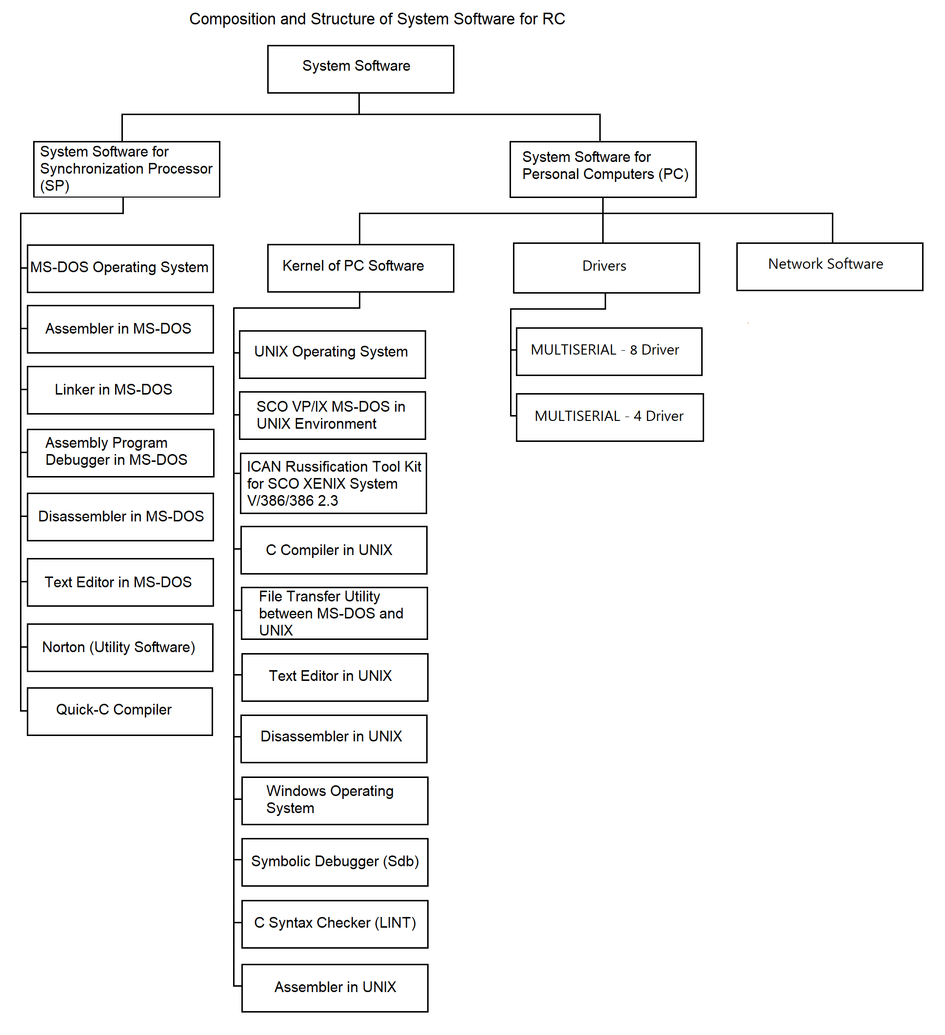
Figure 3.2

In addition to the UNIX OS, the standard PC software includes system utility programs, compilers, and other software development tools used for the development and debugging of RC software:

• SCO VP/IX MS-DOS in the UNIX environment — an MS-DOS emulator under UNIX OS;
• ICAM Russification Tool Kit for SCO XENIX System V/286/386 2.3, intended for localizing OS utilities into Russian;
• C compiler for UNIX;
• File transfer utility between MS-DOS and UNIX environments;
• Text editor in UNIX;
• Reassembler in UNIX used for reassembling standard driver programs in the UNIX OS;
• X-WINDOW — a software suite facilitating the development of efficient human-machine interfaces;
• Symbolic debugger Sdb used to improve error detection and correction during software development in C under UNIX;
• C file syntax checker LINT for identifying syntax errors;
• Assembler translator for UNIX, used in driver development.

An essential component of the PC system software is the set of drivers:

• MULTISERIAL-8 driver;
• MULTISERIAL-16 driver.

For organizing communication between the PC and the SP, a standard terminal driver is planned. This driver supports the MULTISERIAL-8/16 multiplexer. During development, the feasibility of implementing custom drivers for required exchange protocols with the SP will be evaluated. This will be considered if the performance of the standard terminal driver is insufficient to meet technical specifications.

Another component of the system software is network software. The primary network function is transporting data over communication lines between multiple RCs and the central hub, and vice versa.

In the network portion of the “Collection” system, the TCP/IP protocol suite is used as the main tool under the UNIX OS environment.

The TCP/IP suite is a software package consisting of two interconnected protocols:

• IP — Internet Protocol;
• TCP — Transmission Control Protocol.

The primary function of the IP protocol is to deliver data blocks called datagrams from source to destination. A datagram includes header information (for routing) and a data section. If necessary, IP supports datagram fragmentation and reassembly according to the physical network properties. Fragments may arrive out of order and are reassembled accordingly. If any fragment is lost, the entire datagram is considered lost, which raises reliability concerns.

The TCP protocol operates above the IP protocol and enables sending and receiving variable-length segments encapsulated within IP datagrams. TCP’s goal is to establish reliable communication between process pairs. Reliability is ensured through checksum validation, error code return, byte-level sequencing, and acknowledgment requirements. A copy of each segment is queued for retransmission and a timer is started. If acknowledgment is not received in time, the segment is retransmitted.

The transport protocol handles delivery of user data between specific ports (sockets), which serve as access points to the transport service. Communication requires connection setup between two processes, where both sides establish state information. This includes addresses, data sequence numbers, window size (indicating the valid transmission range beyond the last acknowledged byte), forming the structure known as the Connection Control Block. Upon connection termination, resources are released.

Transport-layer protocols must have a unique identifier within the “Protocol” field of the IP header.

3.1.2. System Software of the Synchronization Processor (SP)

The system software of the SP is separated into a dedicated group for the following reasons:

1. The synchronization processor, being a component of the Remote Concentrator (RC), does not have its own operating system, and therefore its software must be developed autonomously under the PC’s OS;

2. The SP software consists of a fairly large set of application programs (drivers, transmission programs, testing, bootloaders, etc.);
3. The technology for SP manufacturing, especially for programming the ROM, is oriented toward using the MS-DOS operating system.

For these reasons, the autonomous software tools used in developing SP software include the following system utilities:

• MS-DOS operating system;
• Assembler compiler for MS-DOS used in SP program development;
• Linker in MS-DOS for building SP application programs;
• Assembly language debugger in MS-DOS for effective debugging of in-development programs;
• Reassembler for rebuilding standard drivers and other programs available only as binary modules;
• Text editor in MS-DOS for preparing SP software documentation;
• NORTON — file management tool;
• Quick-C compiler — used for testing program algorithms.

3.2. Application Software

The application software is intended to perform the functions defined in Section 1. The RC application software can be categorized into three groups by purpose:

• Autonomous;
• Integrated (Complex);
• Service.

3.2.1. Stand-alone Software

The structure of the autonomous software is shown in Figure 3.3. As illustrated, it consists of the following key components:

• Initialization software;
• Software for configuring the RC for a given set of measuring systems (MS);
• RC diagnostic software.

3.2.1.1. Initialization Software

The initialization software prepares the RC for operation. It includes the following program:

• Test program;

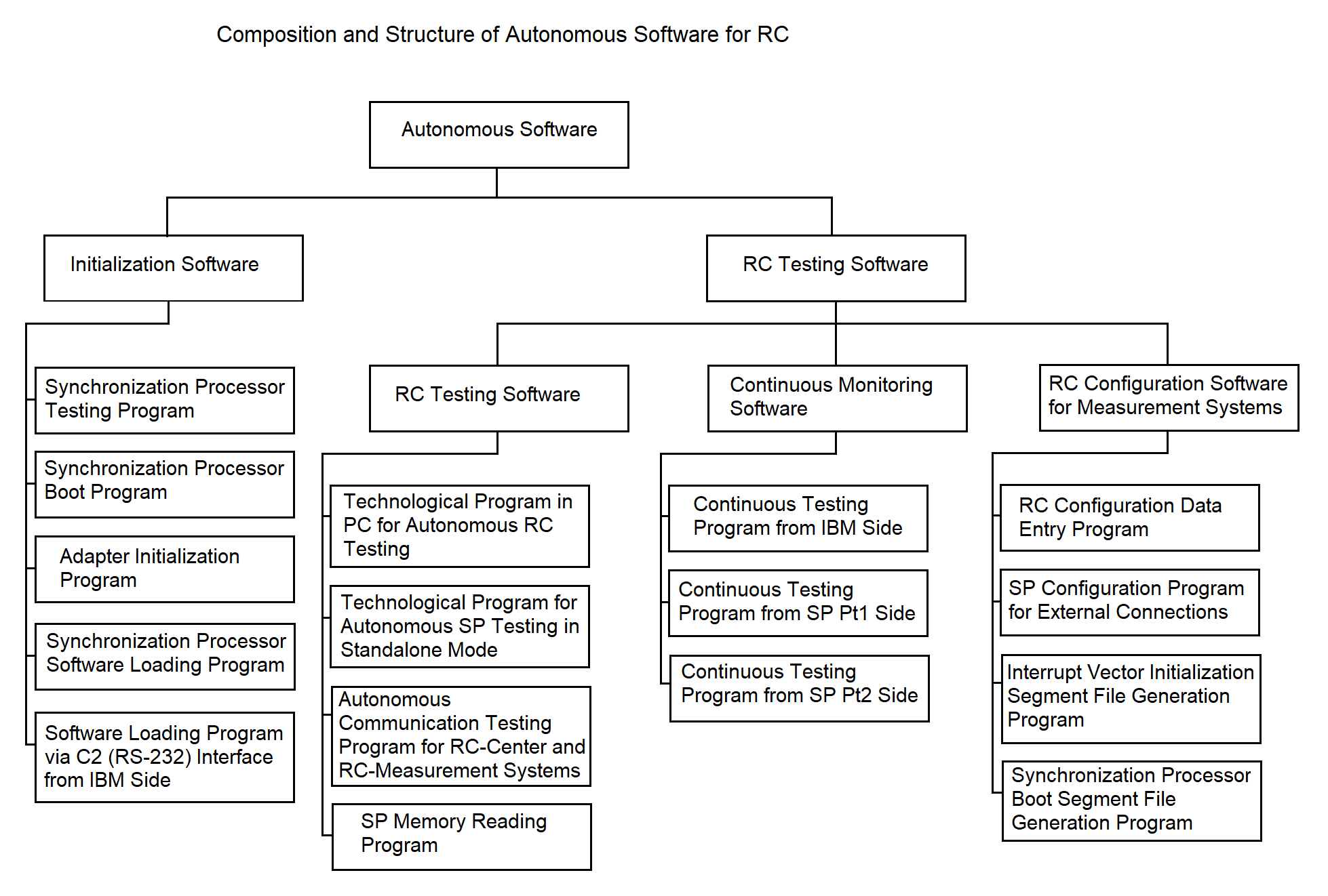
Figure 3.3

Program for loading SP software from the SP side;

Program for loading SP software via the C2 interface from the PC side;

Adapter initialization program.

The test program performs diagnostics of the processors and RAM of the Synchronization Processor (SP) after power-up. This program is hardcoded into the ROM of each SP processor.

The algorithm of the test program is described in section 3.4.1.

The program for loading SP software from the SP side loads programs into SP RAM from the file system located on the PC. It is also stored in the ROM of each SP processor. Loading is done interactively with the loader program via the C2 interface from the PC. The communication protocol during loading complies with GOST 28079-89 (BSC protocol). Loading can be performed over any of the available PC-to-SP communication lines, which may be switched during the process. The loading is done sequentially for each processor, after which the communication lines are released for data exchange.

These loader programs can also read RAM and transmit the data to the PC before transferring control to the application programs. Their operational algorithm is described in section 3.4.2.

The loader program from the PC side uploads SP software and necessary data structures into the SP. All the software and structures are stored in the PC’s file system. The operational algorithm is provided in section 3.4.3.

The adapter initialization program brings the NI599-08 and NI599-06 adapters (part of the SP) into a working state for receiving and transmitting data within the SP. Its algorithm is described in section 3.4.4.

3.2.1.2. Remote Concentrator Configuration Software for IS Composition

This software enables the RC to be customized for different configurations of its interaction with MS (support for BSC protocol, simplex protocol, etc.). The structure is shown in Figure 3.3.

3.2.1.3. Remote Concentrator Diagnostic Software

The structure is shown in Figure 3.3. This software monitors the status of RC hardware. It includes both standalone diagnostics and continuous monitoring components.

The standalone diagnostics software includes the following:

• PC-based diagnostic program for autonomous RC checks;
• SP-based diagnostic program;
• Software for autonomous diagnostics of communication with external nodes (RC–center, RC–MS);
• SP memory reading tool.

The PC-based diagnostic tool is intended for checking RC hardware in standalone mode, e.g., during maintenance. It monitors the PC, SP, their interconnection lines, and SP adapters, and works together with SP-based diagnostic programs.

SP-based diagnostic programs interact with the PC diagnostics. They are based on continuous test programs described in the next section.

The diagnostics for communication with external systems (RC–center and RC–MS) is designed for quick evaluation of the RC’s communication quality. Communication diagnostics with MS assumes supporting software exists on the MS. As such software is currently unavailable, the RC uses a stub instead.

Communication diagnostics with the center can be implemented by file transmission: the center sends a predefined file to the RC, which compares it to a reference. The result determines the communication quality.

The continuous monitoring software verifies SP operation and PC–SP communication during regular RC operations. It is deployed both on the PC and each SP processor.

The SP memory reading tool is a PC-side program that checks SP RAM integrity. It compares the loaded program and data with reference segments on the PC and reports completeness and correctness. The algorithm is not detailed here and will be implemented after finalizing the loader software via C2. A stub is currently used.

The continuous monitoring software includes the following programs:

• Continuous test from the PC side;
• Continuous test from the SP side.

A dedicated communication line between PC and SP is used for these tests. The PC periodically sends a byte to an SP processor. The SP-side test program transfers this byte via shared memory (see section 3.3.5) to the test program of the second SP processor, which returns the byte to the PC via the same line. The PC program compares the received byte with the original and concludes whether the SP is operational. If no response is received within a predefined timeout, the failure is logged with timestamp. More details are in section 3.4.9.

3.2.2. Integrated Software

The integrated software combines programs that support the following Remote Concentrator (RC) functions: receiving data from non-network subscribers, transmitting data into the network, storing data within the RC, managing data streams, receiving data from network subscribers, and transmitting data to the measuring systems (MS).

The main characteristic of the programs included in the integrated software group is that they implement the working modes of the RC. These programs are interrelated in terms of their operations, execution sequence, launch timing, etc.

The integrated software ensures the fulfillment of all target RC functions as specified in the RC software requirements (see Section 1). The structure and composition of the integrated software at the program level (each responsible for a specific target function) are illustrated in Figure 3.4. The components of the integrated software include:

• SP software for communication with non-network subscribers;
• Central dispatcher software for data flow management;
• SP software for communication with network subscribers.

The composition and deployment of the software for communication with network and non-network subscribers are shown in Figure 3.5.

3.2.2.1. SP I/O Software for Communication with Non-Networked Subscribers

Interrupt identification programs for processors 1 and 2

These programs operate within the Synchronization Processor (SP). When a hardware interrupt occurs during data reception, the interrupt is handled by an interrupt processing program. The interrupt handling consists of identifying the data source and launching the appropriate data reception driver for that source. The algorithm descriptions can be found in sections 3.4.12 and 3.4.13.

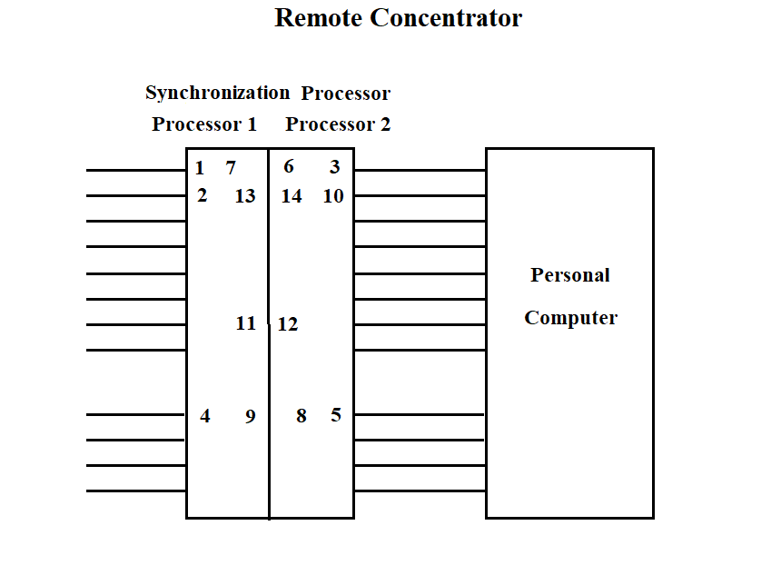
Figure 3.4

1. Driver for receiving Data from "Vega".
2. Driver for receiving Data from "Kama".
3. Driver for receiving Data from PC to "Vega".
4. Driver for receiving Data to SP from the central communication line.
5. Driver for receiving Data from PC to SP (for the central communication line).
6. Program for transmitting Data from "Vega" to PC.
7. Program for transmitting "Vega" Data from SP to PC.
8. Program for transmitting Data from the center to PC.
9. Program for transmitting Data from SP to the center.
10. Program for transmitting Data from "Kama" to PC.
11. Data scanning program in SP Processor 1.
12. Data scanning program in SP Processor 2.
13. Interrupt identification program by Processor 1.
14. Data scanning program in SP Processor 2.

The "Vega" data reception driver is one of the programs operating in the SP, which is called by the interrupt identification program. The call is made by a software interrupt.

The data reception driver places the data into a common area for the two processors, while performing certain actions on the data. A more detailed algorithm is described in section 3.4.14.

The "Kama" data reception driver operates in the SP. The function of the program is to receive data from several "Kama" ISs, prepare the data for transmission to the PC via one of the high-speed lines connecting the SP and the PC. The driver places the data into the common operational memory area for the two processors. The driver algorithm is described in section 3.4.15.

The "Vega" data reception driver from the PC operates in the SP. The driver receives data from the PC and, performing certain actions on it according to the GOST 28079-89 protocol, places it in the common operational memory area for the two processors. The program operation is described in section 3.4.16.

The scanning programs (mailbox scanning by processor 1 and 2) are designed to organize data exchange between the processors. This program scans the common software memory area to identify data intended for transmission from one processor to another. Data transfer to a specific processing program is carried out through a software interrupt mechanism. The program algorithm is described in section 3.4.17.

The "Vega" data transmission program from the SP operates in the SP. The transmission is carried out from the common operational memory area for the two processors to the communication line with "Vega" (see section 3.4.18). The program gains control via a software interrupt from the mailbox scanning program.

The "Vega" data transmission program to the PC operates in the SP. The transmission is carried out from the common operational memory area for the two processors to the communication line with the PC. The transmitted data is prepared in another processor by the "Vega" data reception driver. The program gains control via a software interrupt from the mailbox scanning program. A more detailed algorithm is described in section 3.4.19.

The "Kama" data transmission program to the PC operates in the SP. The transmission is carried out from the common operational memory area for the two processors to the communication line with the PC. The transmitted data is prepared in another processor by the "Kama" data reception driver. The program gains control via a software interrupt from the mailbox scanning program. A more detailed algorithm is described in section 3.4.20.

3.2.2.2. Central Dispatcher Software for Data Flow Management

The central dispatcher software for data flow management, as part of the integrated software, is shown in Figure 3.4. It is designed to accept data flows into the RC, manage the flows, and ensure data storage.

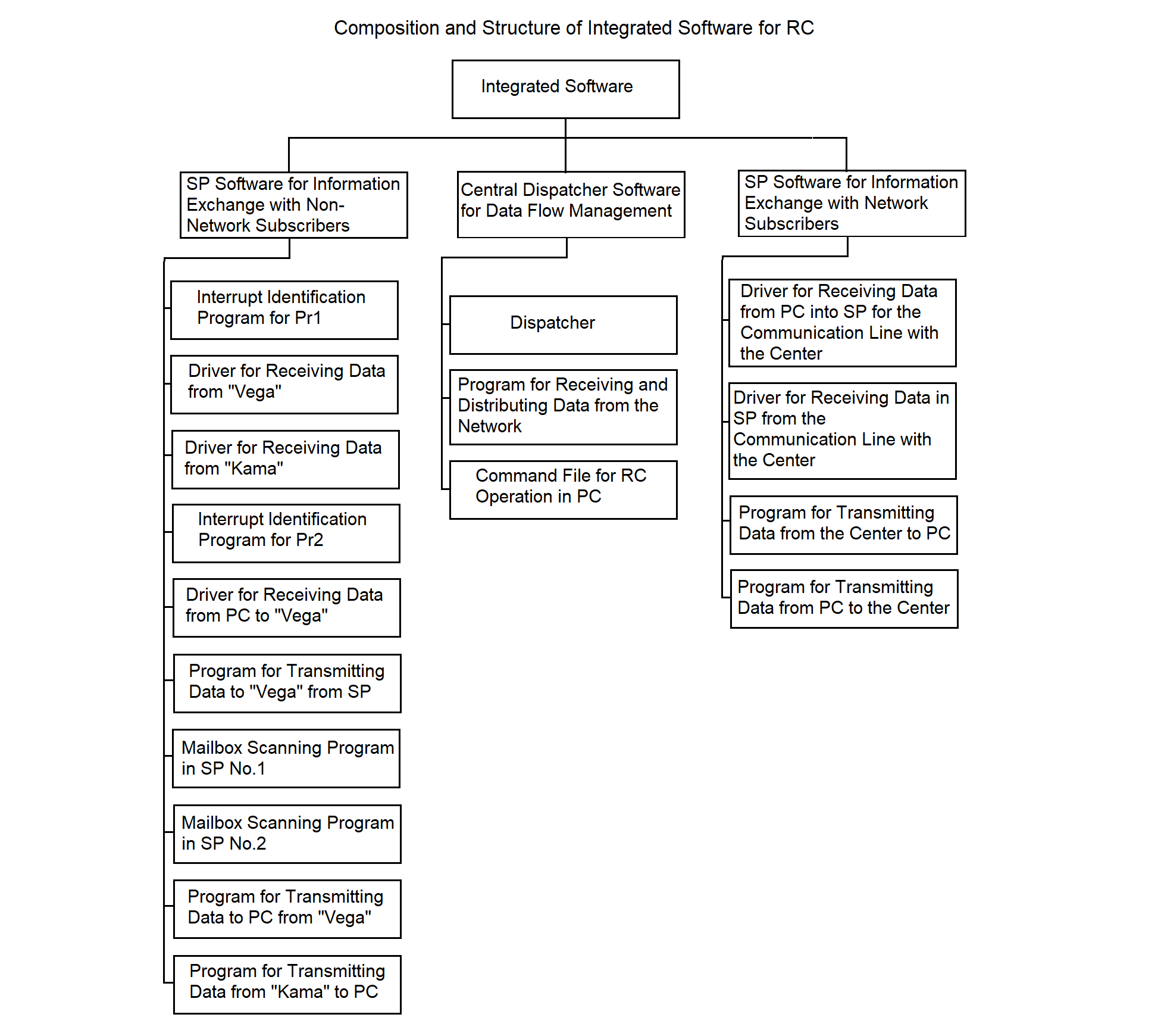
Figure 3.5

The dispatcher program operates in the PC. Its functions include:

• receiving data from ISs in accordance with data exchange protocols;
• transmitting data to ISs;
• transmitting data to the collection center;
• verifying data authenticity;
• registering errors and abnormal situations;
• saving data as files on the HDD.

The implementation method of the dispatcher program, the hierarchy of functions and processes spawned by the program, are described in section 3.4.21.

The program for receiving and distributing data from the network operates in the PC. The functions of the program are similar to the dispatcher's functions. The main difference lies in providing flows from the center to the ISs. See section 3.4.22 for more details.

The command file for RC operation in the PC launches the RC software, starts all necessary processes, and terminates the RC operation.

3.2.2.3. SP Software for Information Exchange with Network Subscribers

The structure of the SP software for information exchange with network subscribers, as part of the integrated software, is shown in Figure 3.4. The software provides data exchange with the center and consists of the following programs:

• driver for receiving data to SP from the central communication line;
• driver for receiving data from PC to SP for the central communication line;
• program for transmitting data from the center to PC;
• program for transmitting data from PC to the center.

All listed programs operate in the SP. Their main purpose is to implement synchronous-asynchronous data conversion (see section 2.1.1).

The driver for receiving data to SP from the central communication line operates in the SP. The driver receives synchronous data, converts it according to the protocol, and writes the data to the common memory area of the processors. The algorithm is described in detail in sections 3.4.23 and 3.4.27.

The driver for receiving data from PC to SP for the central communication line operates in the SP. The driver receives asynchronous data from the PC addressed to the center, converts it according to the protocol, and writes it to the common memory area of the processors. The algorithm is described in detail in sections 3.4.23 and 3.4.28.

The program for transmitting data from the center to PC operates in the SP. The main function of the program is to receive data from the common memory area of the processors and transmit it asynchronously to the PC. The algorithm is described in detail in section 3.4.25.

The program for transmitting data from PC to the center operates in the SP. The main function of the program is to receive data from the common memory area of the processors and transmit it synchronously to the communication line with the center. The algorithm is described in detail in section 3.4.26.

3.2.3. Service Software.

Service software combines programs operating in the SP and the PC and provides solutions to auxiliary tasks that improve the operational characteristics of the RC software:

• analysis of RC operation results;
• display of system operation results;
• control of the delivery set, etc.

The composition and structure of the RC service software are shown in Figure 3.5.

The algorithms of the service software are not considered in this document, as they are developed last, after the implementation of the functional RC software.

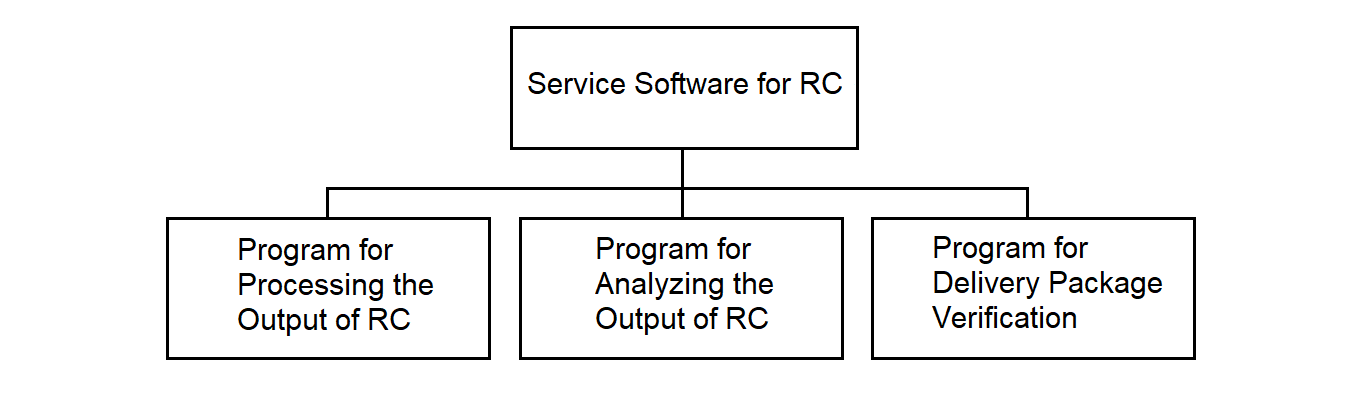
Figure 3.5

The RC result formatting program operates in the PC and is designed for the certification, analysis, and printing of reference data about files containing the RC operation results. Such data can be useful for analyzing the RC operation. The program is implemented as a stub.

The RC operation analysis program operates in the PC. It provides the ability to analyze failure situations during RC operation. The program is implemented as a stub.

The delivery set control program operates in the PC and is designed to ensure control over the contents of the RC delivery set and its integrity.

The program runs before the start of a session and checks the composition of the RC files, compares the checksum of each file with a reference. If deviations are detected, regeneration of the RC is performed. The program acts as an antivirus program. The program is implemented as a stub.

3.3. Remote Concentrator Software Data Structures

This subsection shows the structure of the main data flows passing through the RC, the RC exchange protocol with these flows, as well as the composition and structure of the main data tables of data exchange areas and files used by the RC programs.

3.3.1. Data Structure of IS "Vega"

The data received from the IS "Vega" is represented by a sequence of messages shown in Figure 3.6.

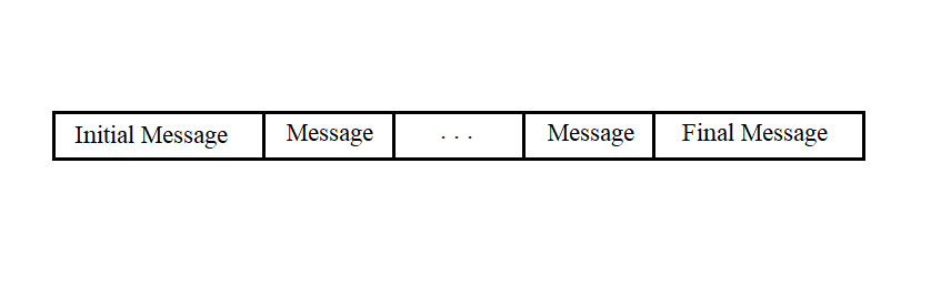
Figure 3.6

Messages of any type consist of a sequence of bytes and can have different lengths. The first five bytes and the last byte of any message have the same fields.

The start and end messages have the structure shown in Figure 3.7.

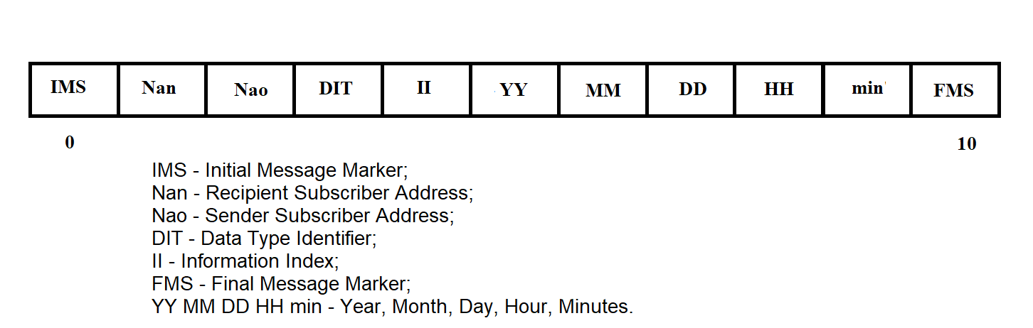
Figure 3.7

The RMB message has the structure shown in Figure 3.8.

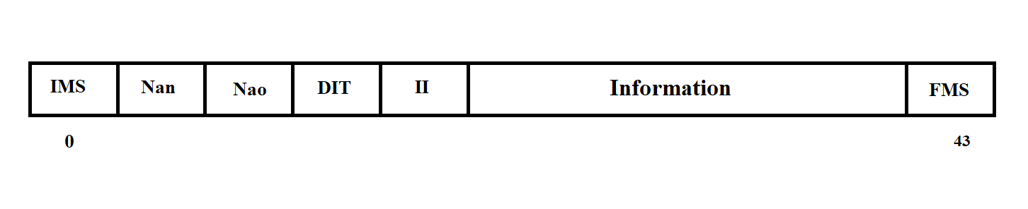
Figure 3.8

The empty RMB message has the structure shown in Figure 3.9.

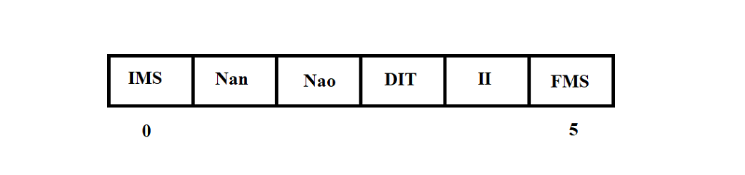
Figure 3.9

Playback mode data messages have the structure shown in Figure 3.10.

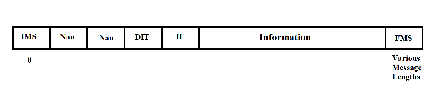
Figure 3.10

Playback mode messages can contain various data and differ in length. The content of any message is determined by its Measurement Information (MI).

The Measurement Information has the following values:

• 1 - initial playback message;
• 2 - processed system data message;
• 3 - message of correlation coefficients of output parameter estimates;
• 4 - message of signal registration times;
• 10 - real-time mode message;
• 11 - initial real-time mode message;
• 12 - final real-time mode message;
• 13 - empty real-time mode message;
• 14 - message of antenna array coordinates;
• 15 - message of information quality reference;
• 16 - message.

Thus, messages with MI 10, 11, 12, 13 are real-time mode messages, and messages with MI 1, 2, 3, 4 are playback messages.

Before transmission to the line, the message from the "Vega" MS is framed with control and error protection symbols in accordance with the GOST 17422-72 exchange protocol (see section 3.3.3).

3.3.2. Data Structure of MS "Kama-A"

The data поступающая from the MS "Kama" is represented by a sequence of messages of the type shown in Figure 3.11.

Figure 3.11

The message consists of a sequence of bits and has a fixed length.

The message begins with a 5-bit marker followed by 60 bits of information. Its structure is shown in Figure 3.12.

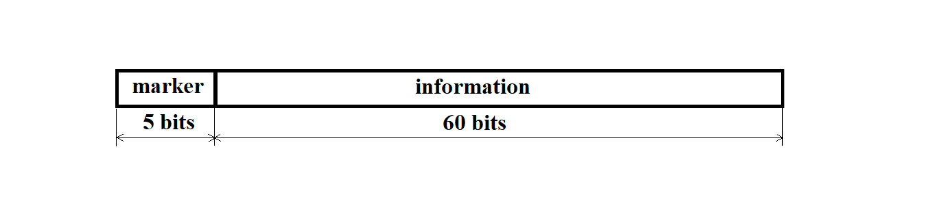
Figure 3.12

The marker has a binary code of 11011.

The message from the MS "Kama-A" arrives at the personal computer from the synchronization processor (SP) as a sequence of 13 bytes.

Here, byte 0 is the message marker, and bytes 1 through 12 contain the actual information.

The structure of the bytes received from the SP is shown in Figure 3.13.

Figure 3.13

Bits 0–4 contain the actual information from the MS "Kama-A", while bits 5–7 indicate the serial number of the MS "Kama-A" from which the message arrived via this channel.

The messages transmitted to the network and stored in the file system of the RC have the structure shown in Figure 3.14.

Figure 3.14

The start-of-message marker and 60 bits of information are packed into 9 bytes of the message from the MS "Kama" in such a way that they form a continuous sequence of bits. As a result, the last 8 bytes each contain only one (least significant) information bit.

3.3.3. Data Exchange Protocol with IS "Vega"

The message text from the "Vega" system is transmitted in transparent mode, i.e., the transmitted information is treated as binary codes.

At the end of each block, a Block Check Sequence (BCS) is transmitted. Cyclic redundancy codes are used with the generator polynomial
X**16 + X**12 + X**5 + 1 as per GOST 17422-72.

3.3.3.1. Control and Service Symbols of the Protocol

Exchange control is carried out using special Service Symbols (SS) and Control Sequences (CS) of symbols selected from the permitted set of GOST 19767-74. Below is a description of the symbols and CS used.

STX — Start of Text.

The STX symbol is sent by the transmitting station at the beginning of the user data text. If the text is divided into blocks, STX is sent at the start of each block. On the receiving side, this symbol (like other service symbols) is not placed into the user's buffer.

ETB — End of Transmission Block.

If the message is divided into blocks, the transmitting station adds this symbol at the end of a data block and then sends the block check sequence. ETB prompts the receiving station to respond.

ETX — End of Text.

The ETX symbol indicates the end of the information message. If the message is divided into blocks, ETX is used to terminate the last data block instead of ETB. The BCS follows the ETX symbol. ETX prompts the receiving station to respond.

EOT — End of Transmission.

By sending EOT (as part of a control sequence), the transmitting station signals the end or suspension of transmission; both stations switch to line monitoring state.

The receiving station may also send EOT to indicate that it is unable to continue receiving data.

ENQ — Enquiry ("Who's there?")

The ENQ symbol is used by the transmitting station in several situations.

Before starting message transmission, the transmitting station uses ENQ to inquire whether the receiving station is ready. Sending ENQ at the end of a data block (instead of ETB or ETX) indicates that the block should be ignored. After sending a data block, the transmitting station uses ENQ to prompt the receiver for a response (if there is no response within a certain time frame) or to repeat the last response.

AR10 — Even Positive Acknowledgement

The sequence of symbols DLE and 0 is used by the receiving station in two cases:

• In response to the initial ENQ — to inform the transmitter of readiness to receive;
• In response to each even-numbered block — if the block was received successfully and the receiver is ready for the next one.

AR11 — Odd Positive Acknowledgement

Sent by the receiving station in response to each odd-numbered block if it was received successfully and the receiver is ready for the next one.

NAK — Negative Acknowledgement

In response to the initial ENQ, the receiving station informs the transmitter that it is not ready to receive the message. During transmission, the receiving station uses NAK to indicate that the last block was received with errors and requests retransmission.

SYN — Synchronization

The SYN control symbol is used to establish and maintain synchronization between stations. At least two consecutive SYN symbols are sent before each information block and before each control sequence. Additionally, the transmitting station sends SYN to the receiver at least once per second during transmission.

DLE ; — Receiver Delay

The receiving station uses the sequence DLE ; to indicate that the last block was received correctly but it is temporarily not ready to accept the next one.

STX ENQ — Transmitter Delay

The transmitting station sends the sequence STX ENQ instead of the next block to indicate a temporary inability to transmit. The receiver should respond with NAK and wait for transmission to resume.

DLE < — Change of Transmission Direction

The receiving station sends the sequence DLE < instead of a positive acknowledgment to an initial request or the next data block if a higher-priority message is pending and it wants to change the direction of transmission.

Since transparent transmission may lead to user data matching control symbols, the following escape sequences are used, inserting DLE before the control symbols STX, ETB, ETX, ENQ, and SYN:

DLE STX — Start of transparent text,

DLE ETB — End of transparent text block,

DLE ETX — End of transparent text,

DLE ENQ — Ignore this transparent text,

DLE SYN — Synchronization within transparent text transmission.

If it is necessary to transmit a DLE character as part of user data, it is doubled.

On the receiving side, additional DLE characters (as well as control symbols) are removed.

3.3.3.2. Formats of Information and Control Sequences

The following notations are adopted:

• SYN — SYN codes;
• FF — Byte of ones;

Figure 3.15

The control sequences are shown in Figure 3.16.

Figure 3.16

3.3.3.3. Basic Exchange Procedures

The main exchange procedures are schematically illustrated below.

For simplicity, the full format of data and control sequences is not shown.

Normal message transmission is shown in Figure 3.17.

Figure 3.17

A request without a response is shown in Figure 3.18.

Figure 3.18

The contention mode (mutual initiative) is shown in Figure 3.19.

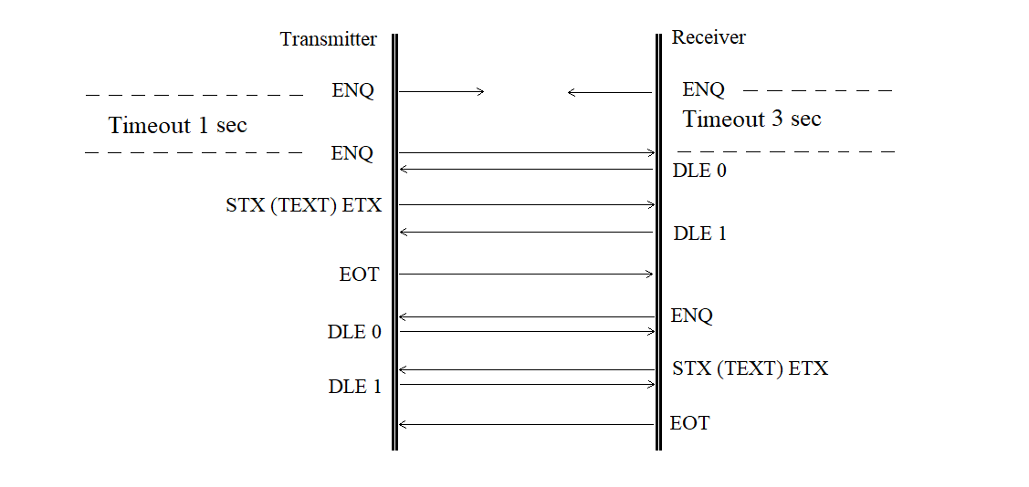
Figure 3.19

The retransmission of a block received with an error is shown in Figure 3.20.

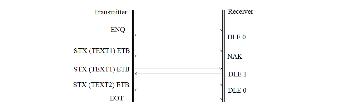
Figure 3.20

The retransmission of a rejected block is shown in Figure 3.21.

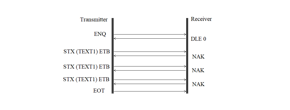
Figure 3.21

The receiver delay request is shown in Figure 3.22.

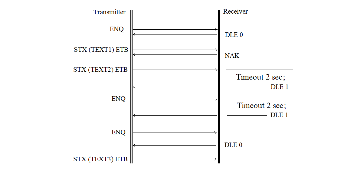
Figure 3.22

The transmitter delay request is shown in Figure 3.23.

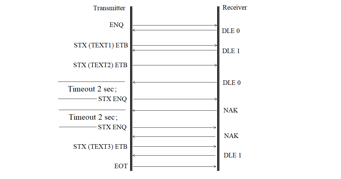
Figure 3.23

The format error is shown in Figure 3.24.

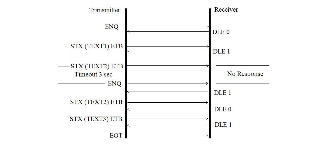
Figure 3.24

The acknowledgement sequence error without correction is shown in Figure 3.25.

Figure 3.25

The acknowledgement sequence error with correction is shown in Figure 3.26.

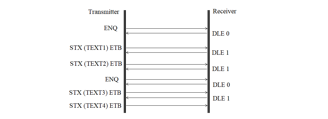
Figure 3.26

The receiver does not respond is shown in Figure 3.27.

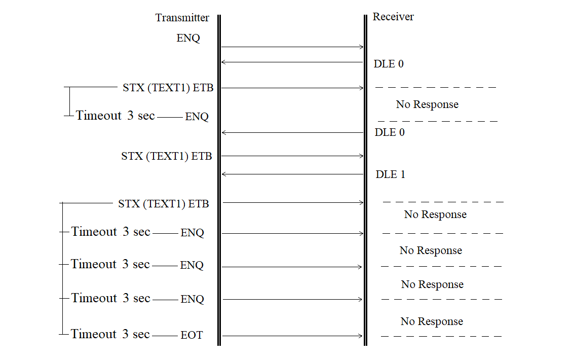
Figure 3.27

The transmitter does not continue transmission is shown in Figure 3.28.

Figure 3.28

The transmitter-side buffer error is shown in Figure 3.29.

Figure 3.29

The transmitter-side external device error is shown in Figure 3.30.

Figure 3.30

Buffer error or overflow, or external device error

on the receiver side is shown in Figure 3.31.

Figure 3.31

Change of transmission direction is shown in Figure 3.32.

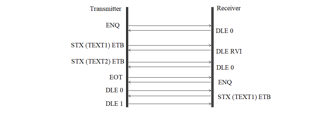
Figure 3.32

3.3.3.4. Formation of Block Check Sequences

The formation of the BCS must begin after the first control character of the block — STX or the control sequence DLE STX. These control characters or control sequences at the beginning of the block must not be included in the BCS calculation.

During the formation of the BCS, all characters transmitted after the initial control character or control sequence of the data block up to the final character (ETB or ETX) in the standard mode, or up to the final control sequence (DLE ETB or DLE ETX) in the code-independent mode, must be included, except:

1) SYN characters in the standard mode or DLE SYN sequences in the code-independent mode;

2) the first DLE character in the control sequences DLE ETB, DLE ETX, or DLE DLE.

The BCS must be transmitted immediately after the control character ETB or ETX in the standard mode, or after the control sequence DLE ETB or DLE ETX in the code-independent mode.

3.3.4. Exchange Protocol with MS "Kama-A"

The process of transmitting measurement data from MS "Kama-A" to the PC occurs in simplex mode. Therefore, no exchange protocols are supported between the PC and MS "Kama-A".

3.3.5. Data Organization of the Synchronization Processor Software

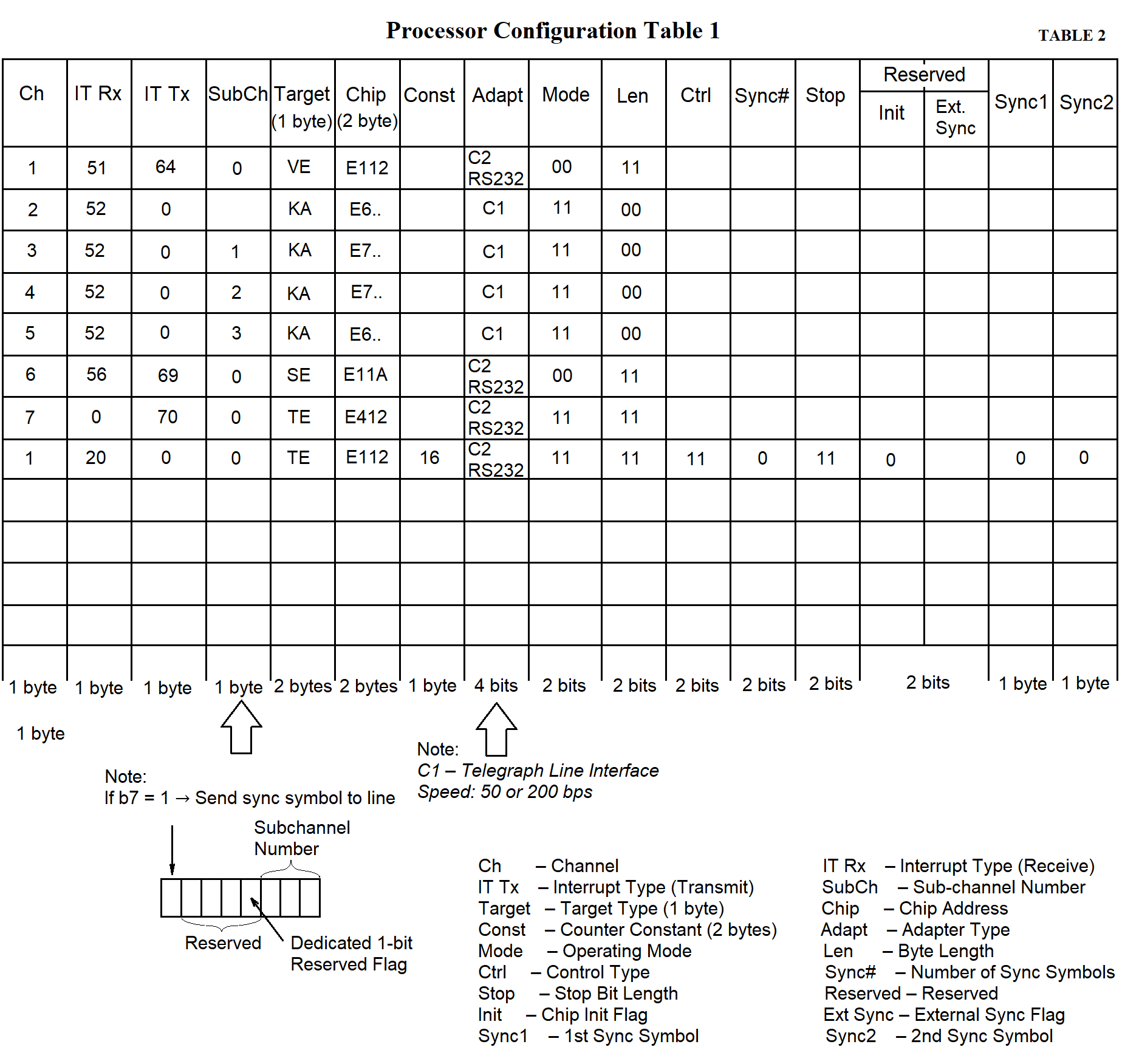
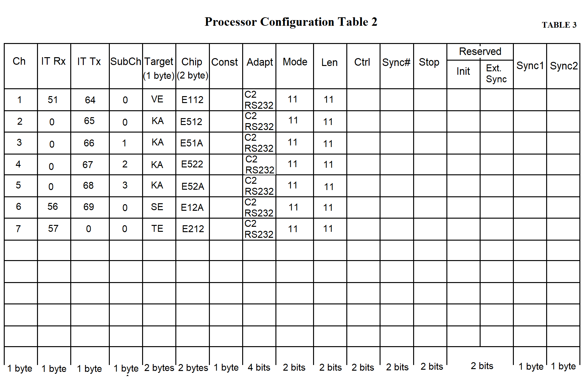
For the proper operation of the SP software, the SP's RAM must be allocated, and space must be reserved for the data (see Table 1).

SP data is organized in tables and memory areas used by the SP software to interact with communication lines — both between lines and between processors.

The main types of SP data are as follows:

• Interrupt vector type tables for each SP processor;
• Processor configuration tables;
• Mailboxes (MB) in the system shared RAM area;
• SP software loading semaphore.

The concept of an "information channel" is introduced. This concept does not imply any physical devices. It refers to any specific stream of data either from a measuring system (MS) or from the data collection center. A channel is understood as a flow of information passing through the MS in either direction. Using this concept, the input and output addresses of the MS and the PC are logically linked. Channel numbers can be assigned arbitrarily, for example, by matching them with the row numbers in the process configuration table.

The subchannel number is used to identify data from multiple "Kama" systems. Each byte from "Kama" is 5 bits long, which means 3 bits remain unused and can be used to identify up to eight MS devices of the "Kama" type. This allows data from eight "Kama" systems to be transmitted to the PC via a single telephone line and then separated within the PC.

The counter constant determines the data transmission/reception speed. Two bytes are allocated for the counter constant in the processor configuration table. The constant is defined as a two-byte hexadecimal number (see page 74, Table 3 in Section 3).

Two bytes are allocated for the chip address in the processor configuration table. The chip address is described as a four-character hexadecimal number. The lower byte specifies the offset relative to the block address. In the upper byte, the lower four bits define the block number (1–5 for NI599-08 blocks, 6–10 for NI599-06 blocks). The upper four bits must contain the hexadecimal value F.

The term "addressee" refers to the type of MS (e.g., Vega, Kama), as well as the network and the continuous testing channel. A one-byte value corresponding to the addressee type is recorded in the table.

Adapters can be of two types:

• C1 (0001);
• C2 (0011).

Four bits are allocated for the adapter type in the process configuration table. The adapter type is represented by a single hexadecimal digit.

The chip operating mode can be:

• Synchronous (00);
• Asynchronous (11).

Two bits are allocated for the operating mode in the processor configuration table.

The byte length can be:

• 5 (00);
• 8 (11).

Two bits are allocated for the byte length in the processor configuration table.

There are two types of parity control:

• Even parity (11);
• Odd parity (01).

Two bits are allocated for the parity control type in the processor configuration table.

When operating in synchronous mode, the number of sync characters is specified:

• One sync character (01);
• Two sync characters (11).

Two bits are allocated for the number of sync characters in the processor configuration table.

The following sync characters may be used:

• SYN;
• DLE SYN;
• DLE STX.

One byte is allocated for each sync character in the processor configuration table. A hexadecimal code of the sync character is recorded in the table.

The stop bit length can be:

• Two bits (11);
• One and a half bits (10);
• One bit (01).

Two bits are allocated for the "stop bit length" column in the processor configuration table.

Two bits are also allocated for the "reserved" column in the processor configuration table.

The total length of the processor configuration table is 169 bytes, as specified in Tables 2 and 3.

Tables 2 and 3 provide example configurations for processors of an RC working with one "Vega" and four "Kama" systems. Row 1 in both tables contains data for the "Vega" MS, rows 2–5 — for "Kama" MS devices, row 6 — for the network, and row 7 — for the continuous testing channel.

3.3.5.3. Mailbox Area

To ensure coordinated processor operation in the SP, data is transferred through a shared memory area. Mailboxes (MB) are located in this shared memory, where one processor writes information and another reads it. Each MB is divided into two parts. The MB is used to support the information channel. Opposing data flows of a single channel pass through their respective parts of the MB (Figure 3.33).

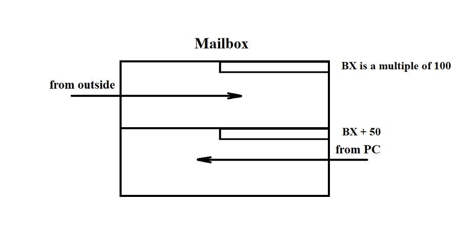
Figure 3.33

For example, the communication channel with the "Vega" MS involves synchronous half-duplex data transmission. Therefore, the first part of the MB can be used to transmit messages from "Vega", and the second part — to transmit acknowledgements to "Vega". Similarly, the MB can be used for any other channel.

To support multiple channels, it is convenient to arrange all MBs consecutively in memory without gaps. In this case, a base address (let's call it BOX) can be used to access the MBs. For clarity, each MB is assigned a number according to its offset from the base address BOX. To ensure that programs "understand" uniformly which MB corresponds to which entity, the MB number is assumed to match the channel number from the processor configuration tables.

Based on the RC architecture, the maximum number of MBs (equal to the maximum number of information channels and thus the number of rows in the processor configuration table) is 13.

Each of the two parts of an MB includes a data presence indicator bit. This is the least significant bit in the least significant byte of each MB part. If the bit is set, the data is present in that part of the MB. If cleared, no data is present. Each part of the MB is allocated 56 bytes (although the SP RAM allows for a larger size) (see Figure 3.34).

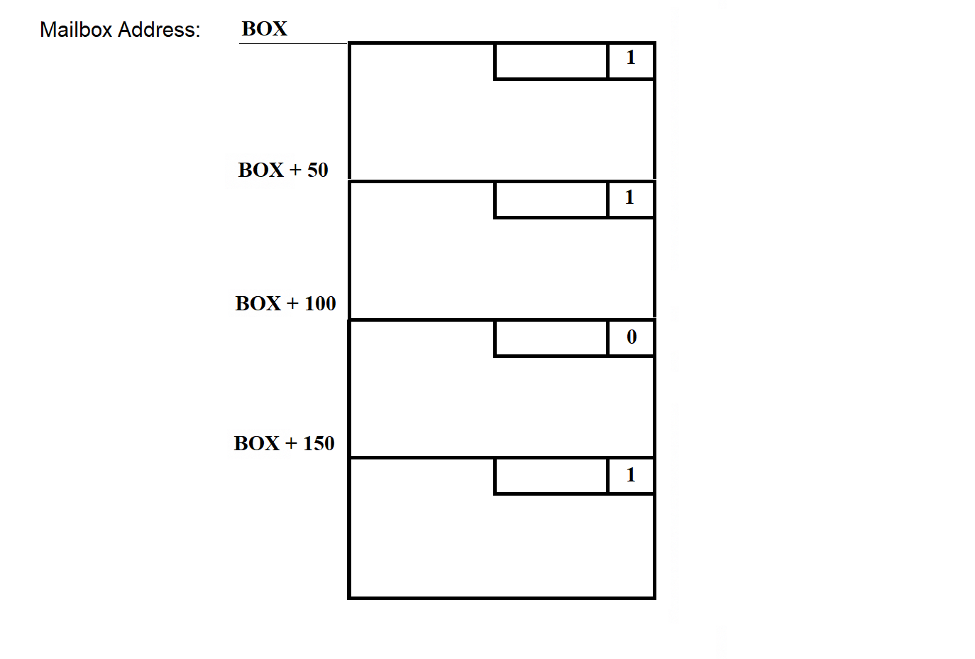
Figure 3.34

The least significant byte of each MB is called the status byte. It stores flags used by the programs that work with the MB. The least significant bit of each status byte is reserved as the data presence bit.

3.3.5.4. Mailbox Usage Concept

To ensure that the data structure is independent of the storage method and to facilitate data exchange between processors, a ring buffer is used. SP software programs access the MBs through standard procedures:

• Read a byte from the buffer
• Write a byte to the buffer

The ring buffer has a "head" — the position where data is written, and a "tail" — the position where data is read. The ring buffer is illustrated in Figure 3.35.

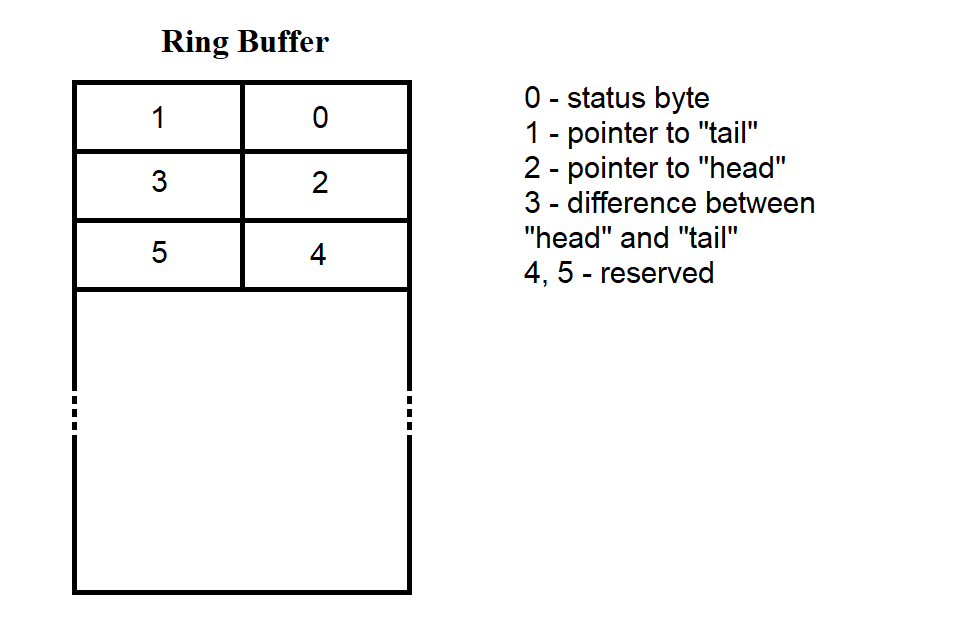
Figure 3.35

The first six bytes contain service information. In each 50-byte part of the MB, 44 bytes are allocated for data. According to Figure 3.35, buffer loading begins with the cell following the fifth byte. When the end of the MB is reached, new bytes are again written starting from the byte after the fifth. During write/read operations, positions 1, 2, and 3 are used to track the "tail," "head," and the difference between them.

Conditions for the correct operation of the ring buffer:

• The "tail" must not overtake the "head".

• The difference between the "head" and "tail" must not exceed the physical length of the buffer (44 bytes).

The state of the MB part before data is loaded into it is shown in Figure 3.36. This situation occurs immediately after the SP software is loaded into SP RAM.

3.3.6. Segment Loading Structure

The data and programs loaded into the SP from the PC side are stored in files on the PC's hard disk. Information about these files is collected into a table stored in the segment file on the same disk. The structure of the segment file is described in section 3.3.7.

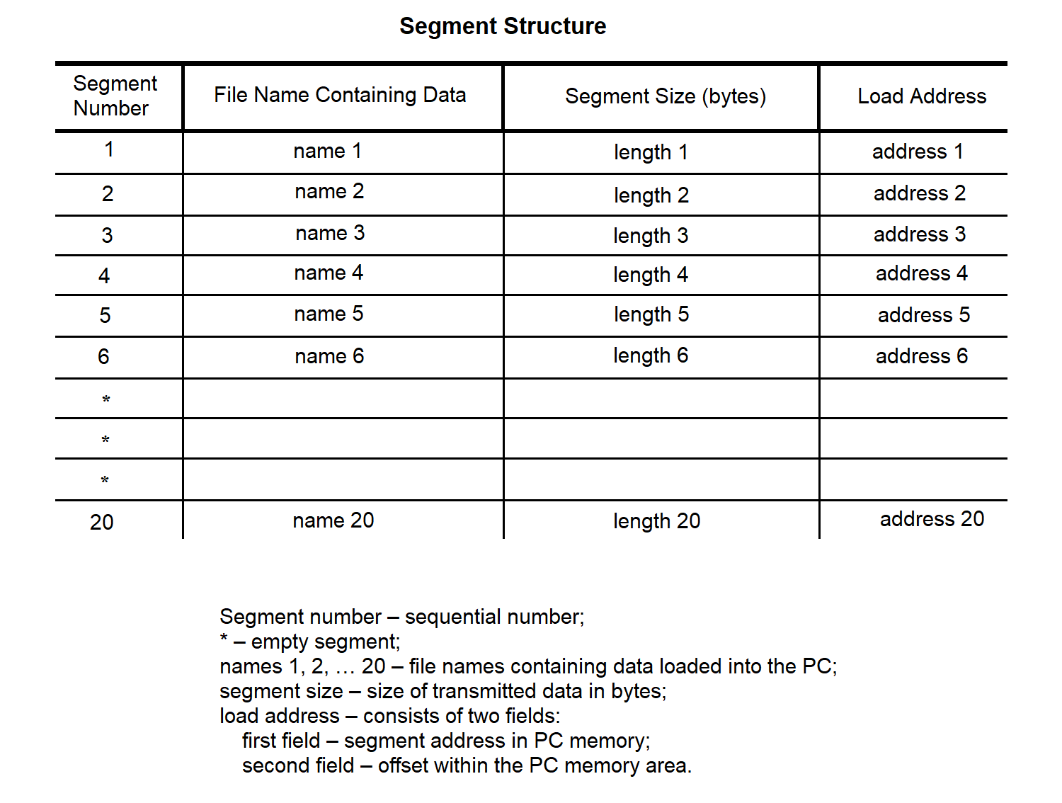
Figure 3.37

All data transmitted to the SP is divided into messages. Each message contains data from a single file.
The message structure is shown in Figure 3.38.

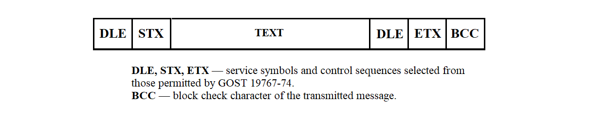
Figure 3.38

The formation of this sequence is described in section 3.3.3.4.
The structure of the transmitted message text may take one of three forms, depending on the required action: reading, writing, or launching a program for execution. The action to be performed is specified by the transfer type indicator, which can take the following values (with respect to NI 526A):

• 2 — transmit data;
• 3 — receive data;
• 4 — launch a program for execution.

The structure of a transmission message is shown in Figure 3.39.

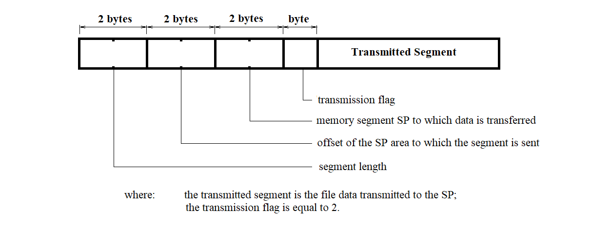
Figure 3.39

The structure of a program launch message is shown in Figure 3.40.

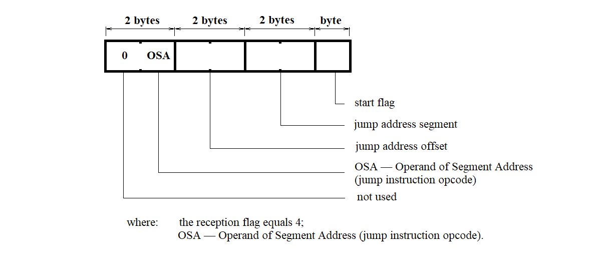
Figure 3.40

The structure of the memory read request message for the control system is shown in Figure 3.41.

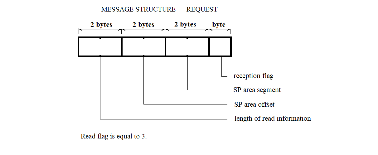
Figure 3.41

3.3.7. Remote Concentrator File System

The segment loading file defines the correspondence between segment numbers, filenames containing the data to be loaded into the SP, and the addresses in the SP memory where this data should be loaded.
The segment loading file is an array of structures of the following type:

            struct {
                char ;   /* Segment number */
                int  ;   /* Address where loading is performed */
                int  ;   /* Offset in the segment where loading is performed */
            };
            

The "MP Configuration" file defines the correspondence between multiplexer line numbers and MS devices.
The "MP Configuration" file is an array of structures of the following type:

            struct {
                char ; /* Multiplexer line number */
                char ; /* MS type: 0 - no MS; 1 - MS "Vega"; 2 - MS "Kama";
                           3 - network; 4 - test line */
            };
            

The interrupt vector initialization segment file defines the correspondence between interrupt numbers and the addresses where the corresponding interrupt handling routines are located.
The interrupt vector initialization segment file is an array of structures of the following type:

                struct {
                  char ; /* Interrupt vector number */
                  int  ; /* Address of the interrupt handler program segment */
                  int  ; /* Offset within the interrupt handler program segment */
                };
            

The processor segment file defines the correspondence of the logical channel for SP processors at the input and output of the SP, and also contains other information required for SP hardware initialization.
The processor segment file is an array of structures of the following type:

                struct {
                  char ;       /* Channel */
                  char ;       /* Receive interrupt type */
                  char ;       /* Transmit interrupt type */
                  char ;       /* Subchannel number */
                  char ;       /* Counter constant */
                  int  ;       /* Chip address */
                  char [2];    /* Addressee */
                  struct {
                    unsigned : 4; /* Adapter type */
                    unsigned : 2; /* Operating mode */
                    unsigned : 2; /* Byte length */
                    unsigned : 2; /* Parity control type */
                    unsigned : 2; /* Number of sync characters */
                    unsigned : 2; /* Stop bit length */
                    unsigned : 2; /* Reserved */
                  };
                  char ;       /* First sync character */
                  char ;       /* Second sync character */
                };
            

A separate processor segment is created for each processor.

The shared memory image segment file is an array of 50-byte records, with a total of 26 elements. In each record, the second and third bytes are initialized to the value 6, while all other bytes are set to 0.

SP software files are files containing the binary images of programs to be loaded into the SP. These files are the result of compilation from C and assembly language sources.

Information received from MS devices is stored in the RC file system. When organizing the storage of incoming MS data, the message-handling programs create a dedicated file for each MS with a unique name. The filename for a given MS is generated according to the scheme shown in Figure 3.42.

Figure 3.42

The RC error log file contains information about the type of error and the time the error occurred during the operation of the RC software.
The RC error log file is an array of structures of the following type:

                struct {
                  char ; /* Error type: 0 - SP continuous test error */
                         /* 1 - no communication line with CC */
                  long ; /* Error occurrence time in seconds since */
                         /* 00:00:00 January 1, 1970 (UTC) */
                };
            

3.4. Remote Concentrator Software Operation Algorithm

3.4.1. Synchronization Processor Test Program

The testing and initialization of the synchronization processor are performed according to a predefined sequence of steps:

1. Microprocessor register test;
2. ROM test;
3. RAM test;
4. Programmable interrupt controller test;
5. Timer test;
6. Test of chip 580VV51;
7. Timeout test;
8. Interrupt vector setup;
9. Interrupt mask setup for the programmable interrupt controller;
10. NI599-03 unit test;
11. Initialization of NI599-08 units;
12. Waiting for connection via RS232 channel.

All of the above actions are performed regardless of any fault conditions that may occur. The test progress is displayed via the indicators on the NI599-31 unit. Turning off any LED, except for LED "0", indicates the successful completion of the corresponding test. Turning off LED "0" signals the start of testing. Turning it on indicates successful completion of the entire test procedure.

The test and initialization programs are stored in the ROM of the NI599-31 unit in the following sequence:

• NI599-31 unit test;
• Interrupt vector loader;
• NI599-03 unit test;
• IRPS driver;
• RS232 driver;
• Checksum area.

The memory size occupied by these programs and their address locations will be defined during the software development stage.

After completion of testing and initialization, two hardware interrupts are enabled in the MCC:

• IRQ1 — timeout;
• IRQ2 — “receiver ready” signal from the IRPS channel.

Access to the IRPS driver and communication protocols are described in document AFKE.40003-01-31-31.

3.4.2. SP Software Loading Program (from SP side)

The SP software loading program, executed from the SP side, supports a communication protocol over the C2 interface that is similar to the BSC transparent mode protocol (according to GOST 28079-89). It is designed for loading programs and data into the resident and system memory of the NI526A device via one of the channels of the NI599-08 units, operating in asynchronous mode at a speed of 9600 bps.

The SP software loading program from the SP side performs the following functions:

• Initialization of NI599-08 units;
• Receiving data from the communication line into the resident and system memory of the NI526A device at a specified address;
• Transmitting data from the resident and system memory of the NI526A device to the communication line with the PC at a specified address;
• Issuing a jump instruction to the processor at a specified address;
• Verifying the correctness of the received data;
• Generating and sending confirmation messages over the communication line about the correctness of the received data.

SP Software Loading Program (from SP side)

The SP software loading program (executed from the SP side) gains control after the NI599-03 unit test is completed.

Upon receiving control, the program allows the processor to check the initialization flag of the NI599-08 units.

If the flag is not set (i.e., not equal to zero), the processor initializes the NI599-08 units, configuring them for the required operating mode. After initialization is completed, the processor sets the initialization flag to one. It then begins sequential polling of the NI599-08 channels to establish communication via the C2 interface. When a channel that has received a byte from the communication line is detected, the processor switches to the corresponding line-handling subroutine.

The line-handling subroutine is triggered when the processor detects any first channel of an NI599-08 unit that has received a byte from the communication line.

Exit from the line-handling subroutine—and subsequently from the entire SP software loading program—occurs only after the processor receives a text message containing a command to jump to a specified address in the control array. Upon exiting the SP software loading program, the processor releases the bus, allowing another processor to take control, whose loading procedure follows the same sequence.

The sequence of information exchange between the PC and SP, and the SP's response handling, is shown in Figure 3.43.

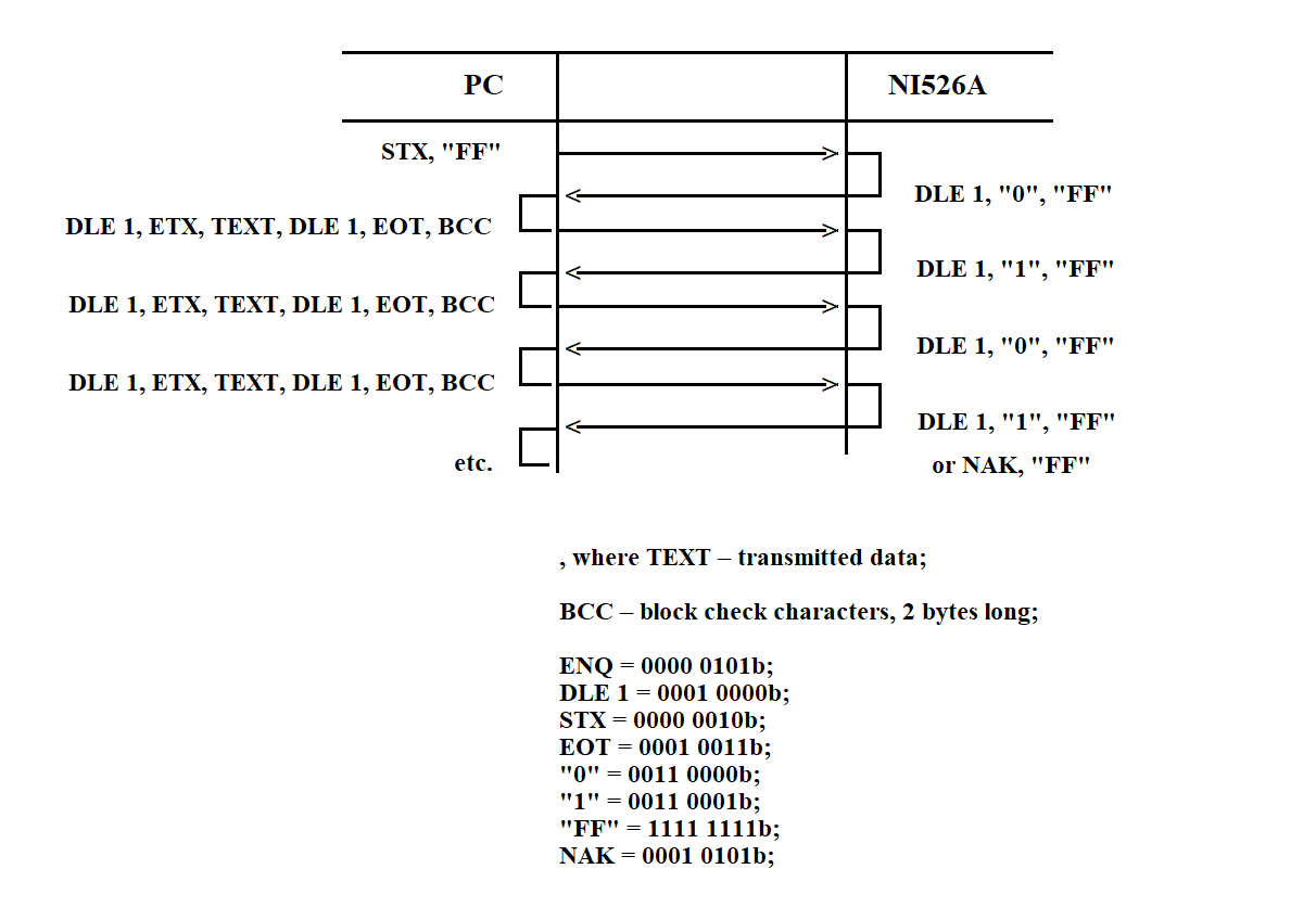
Figure 3.43

When receiving data from the PC, the subroutine calculates the BCS (Block Check Sequence). The calculation starts after receiving the STX byte and ends with the ETX byte (inclusive). In byte sequences such as DLE, DLE and DLE, ETX received within the message text, the first DLE byte is discarded and not included in the BCS calculation.

If the calculated BCS does not match the received one, a response of the form NAK, "FF" is sent over the communication line. During message reception, the processor always analyzes the mandatory control byte array located at the beginning of the message text. Depending on the operation code, it performs one of the following: receiving data, transmitting data, or jumping to a specified address. The structure and location of the control array within the message text are shown in Figure 3.44.

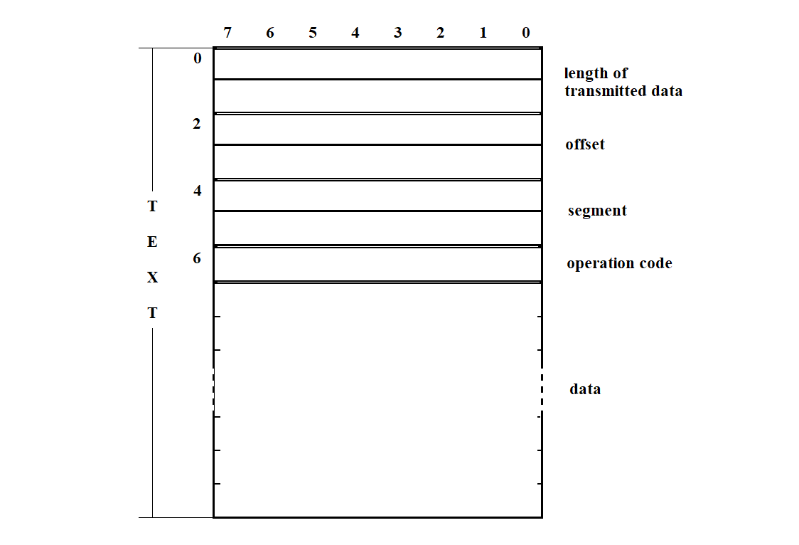
Figure 3.44

The SP software loading program (from SP side) uses the following procedures:

1. Initialize NI599-08 units
2. Reset variables (set 1)
3. Reset variables (set 2)
4. Transmit a data byte to the communication line
5. Receive a data byte from the communication line

PC-side Software Loading Program

1 Reset variables 1
1 IF INITIALIZATION FLAG is not set
INITIALIZE NI599-08 blocks
SET INITIALIZATION FLAG

1 ELSE   /* if INITIALIZATION FLAG is set */
SET CHANNEL COUNTER
READ CHANNEL STATUS WORD

2 IF RECEIVER READY BIT IS SET
RECEIVE DATA BYTE FROM COMMUNICATION LINE

3 IF BUFFER A COUNTER = 2
4 IF FLAG 2 is not set
5 IF FLAG 1 is not set
6 IF BUFFER A = ENQ “FF”
TRANSMIT to communication line DLE “0” “FF”

7 IF BUFFER B COUNTER < 7
Reset variables 2
7 ELSE   /* BUFFER B COUNTER = 7 */

8 IF START FLAG in BUFFER B is set
Reset VARIABLES 1
Jump to start address
Release bus

8 ELSE   /* START FLAG in BUFFER B is not set */
9 IF TRANSMISSION FLAG in BUFFER B is set
Copy first and second byte of BUFFER B to TRANSMISSION LENGTH
10 IF TRANSMISSION LENGTH ≠ 0
Transmit data byte to communication line
Decrease TRANSMISSION LENGTH
10 ELSE  /* TRANSMISSION LENGTH = 0 */
Reset variables 2
10 END-IF
9 ELSE /* if TRANSMISSION FLAG in BUFFER B is not set */
Reset variables 2
9 END-IF
8 END-IF
7 END-IF
6 ELSE   /* BUFFER A ≠ ENQ “FF” */

7 IF BUFFER A = DLE STX
Reset BUFFER A COUNTER
Reset BUFFER B COUNTER
Reset FLAG 1
7 ELSE   /* BUFFER A ≠ DLE STX */
Reset BUFFER A COUNTER
7 END-IF
6 END-IF

5 ELSE   /* FLAG 1 is set */
6 IF BUFFER A = DLE ETX
Reset FLAG 1
Add to BCC the high byte from BUFFER A
Reset BUFFER A COUNTER
Set FLAG 2

6 ELSE   /* BUFFER A ≠ DLE ETX */
7 IF BUFFER A = DLE DLE
Copy high byte of A → low byte
Decrease BUFFER A COUNTER
7 ELSE   /* BUFFER A ≠ DLE DLE */
8 IF BUFFER B COUNTER < 7
Add to BCC the low byte of BUFFER A
Decrease BUFFER A COUNTER
Copy low byte of A → BUFFER B
Increase BUFFER B COUNTER
9 IF BUFFER B COUNTER = 7
Set OFFSET
Set SEGMENT
9 END-IF
8 ELSE   /* IF BUFFER B COUNTER = 7 */
Add to BCC the low byte of BUFFER A
Decrease BUFFER A COUNTER
Low byte of BUFFER A → memory
Increase OFFSET
8 END-IF
7 END-IF
6 END-IF
5 END-IF

4 ELSE   /* FLAG 2 is set */
Reset FLAG 2
5 IF BUFFER A = BCC
Transmit to line DLE “1” “FF”
5 ELSE   /* BUFFER A ≠ BCC */
Transmit to line NAK “FF”
Reset variables 2
5 END-IF
4 END-IF
3 END-IF

2 ELSE  /* RECEIVER-READY = 0 */
Decrease CHANNEL COUNTER
3 IF CHANNEL COUNTER = 0
Set CHANNEL COUNTER
Read channel status word
3 END-IF
2 END-IF
1 END-IF

Procedure: initialize blocks of NI599-08

Set BLOCK COUNTER
IF BLOCK COUNTER ≠ 0
Initialize timers
Initialize channels
Decrease BLOCK COUNTER
END-IF
    

Procedure: Reset Variables 1

Reset BUFFER A COUNTER
Reset BUFFER B COUNTER
Reset FLAG 1
Reset FLAG 2
Reset CHECKSUM
    

Procedure: Reset Variables 2

Reset BUFFER A COUNTER
Reset BUFFER B COUNTER
Reset FLAG 1
Reset CHECKSUM
    

Procedure: Transmit data byte to the communication line

Read CHANNEL STATUS WORD
IF TRANSMITTER READY bit is set
Write data byte to channel data register
END-IF
    

Procedure: Receive data byte from the communication line

Read data byte from channel data register
Copy high byte of BUFFER A to low byte
Copy data byte to high byte of BUFFER A
Increase BUFFER A COUNTER
    

3.4.3. SP Software Loader via Connector C2 (Computer Side)
The SP software loader is designed to load programs and data into the resident and system memory of the NI-526A. It is executed as part of a command file that runs at computer startup.

The loader receives input specifying which files to upload to the SP. Its output consists of messages containing data for loading into the SP and control sequences (CS) that implement the BSC exchange protocol. The loader interacts with the tty terminal driver and performs the following actions:

1) Reads from the computer disk a segment file that contains information about all segments to be loaded into the SP. The structure of this file is shown in Figure 3.37 (see section 3.3.6).

2) For each segment, the loader reads the corresponding file from disk, forms a message for transmission to the SP over the RS232 interface according to the BSC protocol. This communication uses special control characters (CC) and control sequences from the set defined in GOST 19767–74. The formats and definitions of these characters and sequences are detailed in sections 3.3.3.1 – 3.3.3.2. The exchange structure is described earlier in section 3.4.2.

3) Before sending the message, the loader computes the BCC using a CRC with the generator polynomial X¹⁶ + X¹² + X⁵ + 1 (GOST 17422–72, see section 3.3.3.4).

4) The message is transmitted to the SP. After sending, the loader waits for an acknowledgment from the SP software. If successful (DLE "1" or DLE "2" is received), the loader proceeds with the next segment.
If the SP responds with DLE "NO", the segment is retransmitted up to three times. After three failed attempts, an error message is shown on the terminal.

5) After successfully uploading all segments, the loader issues a command to launch the SP software (segment 20). The structure of this command is shown in Figure 3.40 (see section 3.3.6). From this point, the loaded software begins execution in the SP. If the final segment is missing, no launch is performed.

6) The loader provides a verification mechanism to check the integrity of the upload by either reading SP memory or visually inspecting the result. To perform this, a memory-reading program must be implemented on the SP side, and a comparison utility on the workstation. The format for a memory read request message is shown in Figure 3.41 (see section 3.3.6).

In response to the request, the SP loader transmits data from SP memory to a file on the workstation. This file can be displayed on the screen for manual inspection or checked using the comparison utility. The result is shown on the terminal.

Upon startup, the loader sends a DLE 0 control sequence to the communication line and waits for a response from the SP in the form of a DLE 0 control sequence. If no response is received, the request is repeated every 3 seconds, up to 5 attempts. After that, an error message is displayed on the workstation terminal.
The message format is shown in Figure 3.45.

Figure 3.45

This continues until confirmation is received from the SP side, or the operator intervenes in response to the fault message.

Once the connection is established, the loader program immediately begins writing data and programs to the synchronization processor. It opens the segment file and starts the loading procedure. Two operating modes are provided for the loading process: technological and main. The mode of operation can be selected and entered by the computer operator in response to a request of the type shown in Figure 3.46.

Figure 3.46

The diagram of the hierarchy of functions of the loading program is shown in Figure 3.47.

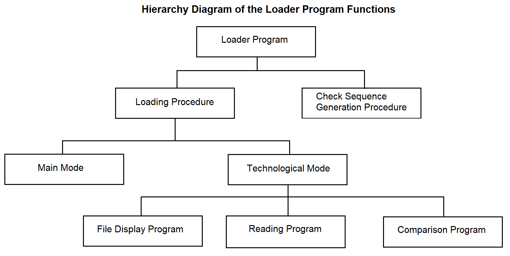
Figure 3.47

In the main mode, the loading procedure reads from the disk each segment subject to loading. To do this, if the segment is not empty, it opens the file whose name is recorded in the segment file table. Its contents are placed into the message buffer (BC). It forms the message text and supplements it with control characters provided by the BSC protocol, as shown in Figure 3.48.

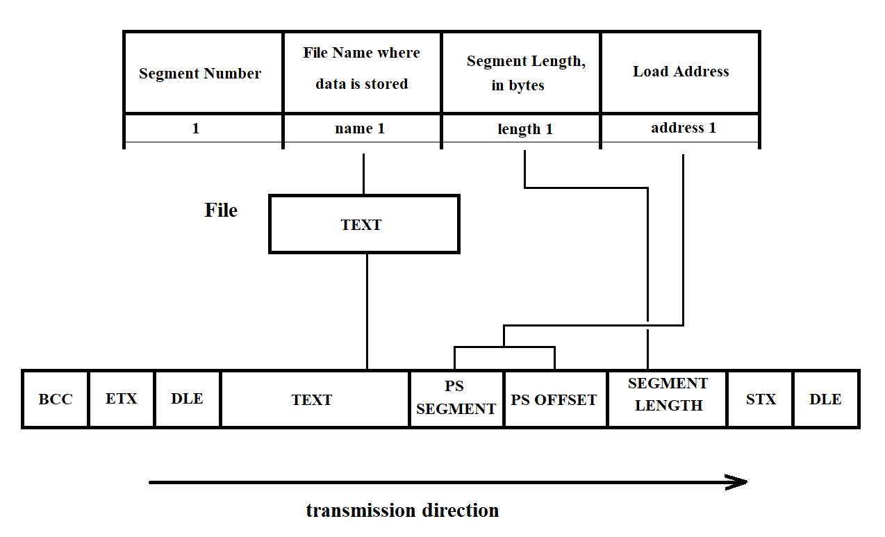
Figure 3.48

If the text contains information corresponding to the DLE character, this character is duplicated. To ensure error-free data transmission, the BCC (Block Check Character) is calculated during the checksum generation procedure.

Then the final message is sent to the terminal driver for further transmission over RS232 to the SP. After this, the loading procedure waits for acknowledgment from the SP: control signal DLE 0 — for each even transmitted message, and DLE 1 — for each odd transmitted message. If the SP sends a control signal "NO", the faulty segment is resent up to three times. After that, an error message is displayed on the terminal. The message format is shown in Figure 3.49. Upon receiving the message, the operator either initiates a repeat load or calls the personnel responsible for performing maintenance work.

Figure 3.49

If the transmission is successful, the loading procedure proceeds to read the next segment (see above). After all segments have been loaded into the SP, the loading procedure sends the final, 20th segment to the SP. This segment contains a command to start the SP software. The structure of the startup message is shown in Figure 3.40 (see section 3.3.6). At this point, the loading of one SP is complete.

Operation in technological mode makes it possible to verify the correctness of the loading by reading the memory and through visual inspection. To do this, after loading all segments except the last one into the SP (see the description of segment loading in the main mode), the operator is prompted with a request in the following format:

Figure 3.50

By default, a full check will be performed for all segments. The following prompt allows you to select the type of check:

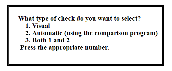
Figure 3.51

After this, the reading program (described below) sends a read request to the SP. The structure of the request message is shown in Figure 3.41 (see section 3.3.6). In response to this request, the loader program located in the SP ensures the transfer of data from the selected segment in SP memory to the PC verification file.

If the operator has selected the visual check, the contents of the verification file are displayed on the screen. In the case of the second type of check, the comparison program is invoked to compare the original file with the verification file. The operator receives a message with the result of the check. If the result is negative, the message has the following format:

Figure 3.52

After that, the operator is prompted:

Figure 3.53

If "yes" is entered, the verification procedure is repeated. If "no", the operator is allowed to load the SP in the main mode.

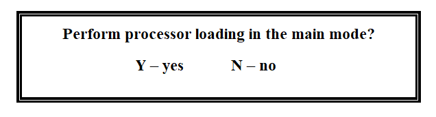
Figure 3.54

If yes, the loading procedure is executed. If not, the SP software loader program finishes its operation.

To operate, the loader program uses the following:

System call:
ALARM – set a process alarm;

Library functions:
FOPEN – open an input/output stream;
FDOPEN – associate a stream with a file descriptor opened by FOPEN;
FCLOSE – close an open input/output stream;
FREAD – read a specified number of bytes from the input stream;
FWRITE – write a specified number of bytes to the output stream;
FGETC – read the next character from the input stream STREAM;
FPUTC – write a character to the stream;

Programs: comparison, displaying file on screen.

Flags:
Start flag (SF) – set upon receipt of DLE0 from the SP, in response to the initial KTM request.
Error-free reception flag (EFRF) – set when sending a request message, reset upon receiving a message without errors. Used by the reading program.
Repeat – used by the loading procedure. Set when sending a message to the SP, reset upon receiving a positive response.

Buffers:
RO – Response Output Buffer: buffer for sending responses to the SP.
MT – Message Transmit Buffer: buffer containing messages to be sent to the SP.
RI – Receive Input Buffer: buffer for receiving data from the SP.

The pseudocode of the program is provided below.

Software Loader Program to SP via C2 interface from the PC

Response counter (RC) is set to 0
Start flag (SF) is cleared

LOOP  /* while there is no response */
IF SF is cleared
ELSE
Start 3-second timer
END-IF

IF response counter is less than 5
ELSE
Display warning on PC screen
Reset counter
END-IF

Send ENQ request to the line
Switch to acknowledgment reception mode
Increment response counter by 1
Set start flag   /* SF = 1 */

END-LOOP

/* When DLE 0 is received – connection established */

Open segment file
Execute loading procedure
Send request to operator on terminal
IF second processor needs to be loaded
Execute loading procedure
ELSE
END-IF

Close segment file
    

Loading Procedure

A := 3
Prompt the operator   /* in which mode to operate */
Assign the response to variable A
Read the first row of the segment table

WHILE sector number (SN) ≠ 20
Repeat := 1
Repeat counter (RC) := 0
IF segment is not empty THEN
Open file
Form message in MT
Form BCC
WHILE Repeat > 0
Send message from MT to the terminal driver
Switch to acknowledgment reception mode from SP
SELECT: response from SP
CASE DLE 0 and DLE 1
RC := 0
CASE NO
RC := RC + 1
IF RC = 3 THEN
Output message to PC screen
END-IF
END-WHILE
END-IF
Read the next row of the table
END-WHILE

IF A = 1 THEN
Execute the procedure for processing the technological mode
ELSE
Read segment 20
Form message in MT
Form BCC
Repeat := 1
WHILE Repeat > 0
Send message from MT to the terminal driver
Switch to acknowledgment reception mode from SP
SELECT: response from SP
CASE DLE 0 and DLE 1
RC := 0
CASE NO
RC := RC + 1
IF RC = 3 THEN
Output message to PC screen
END-IF
END-WHILE
END-IF
    

Technological mode processing procedure

Open verification file
Prompt the operator   /* what type of control */
IF full control THEN
Read the first row of the segment table
Segment counter (SC) := 0
WHILE SC < 20
IF segment is not empty THEN
Execute memory reading program
ELSE
END-IF
SC := SC + 1
END-WHILE
ELSE
Read the N-th row of the table
Execute memory reading procedure
END-IF

Prompt the operator   /* what type of control */
SELECT operator's response
CASE visual
Execute file output program to screen
CASE using comparison program
Execute comparison program
Display result on screen
CASE none of the above
Execute file output program to screen
END-SELECT
    

Memory read procedure

Write to the message buffer:
1. DLE STX
2. Segment length in bytes
3. SP area offset
4. SP area segment
5. Read flag
6. ETX

Compute BCC and write it to the message buffer

Transfer the message from the message buffer to the Synchronization Processor (SP)

Switch to reception mode from SP

Reception Without Error Flag := 1

WHILE Reception Without Error Flag = 1
Receive message into the reception buffer
Compute BCC of the received message
IF the message was received with an error THEN
Send NAK to SP using the response buffer
ELSE
Write the message from the reception buffer to the reception file
Reception Without Error Flag := 0
Send positive acknowledgment using the response buffer
END-IF
END-WHILE
    

3.4.4. Adapter Initialization Program

The adapter initialization program operates within the SP. It is called by the SP software loader from the SP side. The main function of the adapter initialization program is to set the operating modes of the adapters according to the processor configuration table (see Tables 2 and 3). The program sequentially processes the entire table, reads microcircuit addresses, determines the block number and adapter type, and initializes them accordingly (first the block, then the microcircuit). To avoid reinitialization of a block, it is recommended to use the Initialized Block Register (IBR). The structure of the IBR is shown in Figure 3.60.

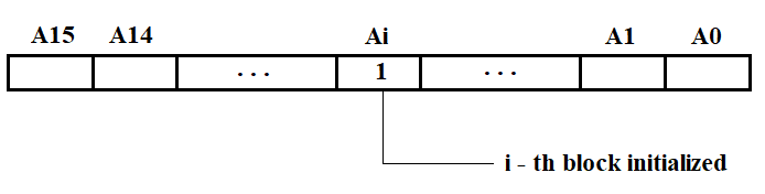
Figure 3.60

The hierarchy diagram of the adapter initialization program functions is shown in Figure 3.61.

The NI526 unit includes modules NI599-06 and NI599-08, intended for interfacing C1 and C2 with VIMK. The NI599-06 module is currently under development. The initialization subroutine for NI599-06 will be developed after receiving the technical documentation for this module.

Each NI599-08 module includes:

• two timers implemented using IC 580VI53;
• four universal synchronous/asynchronous transceivers (USAPP) implemented using IC 580VV51.

The module address is set using jumpers on the printed circuit board.

Module initialization is performed by writing the module control word (MCW) into the corresponding register. The format of the module control word is shown in Figure 3.62.

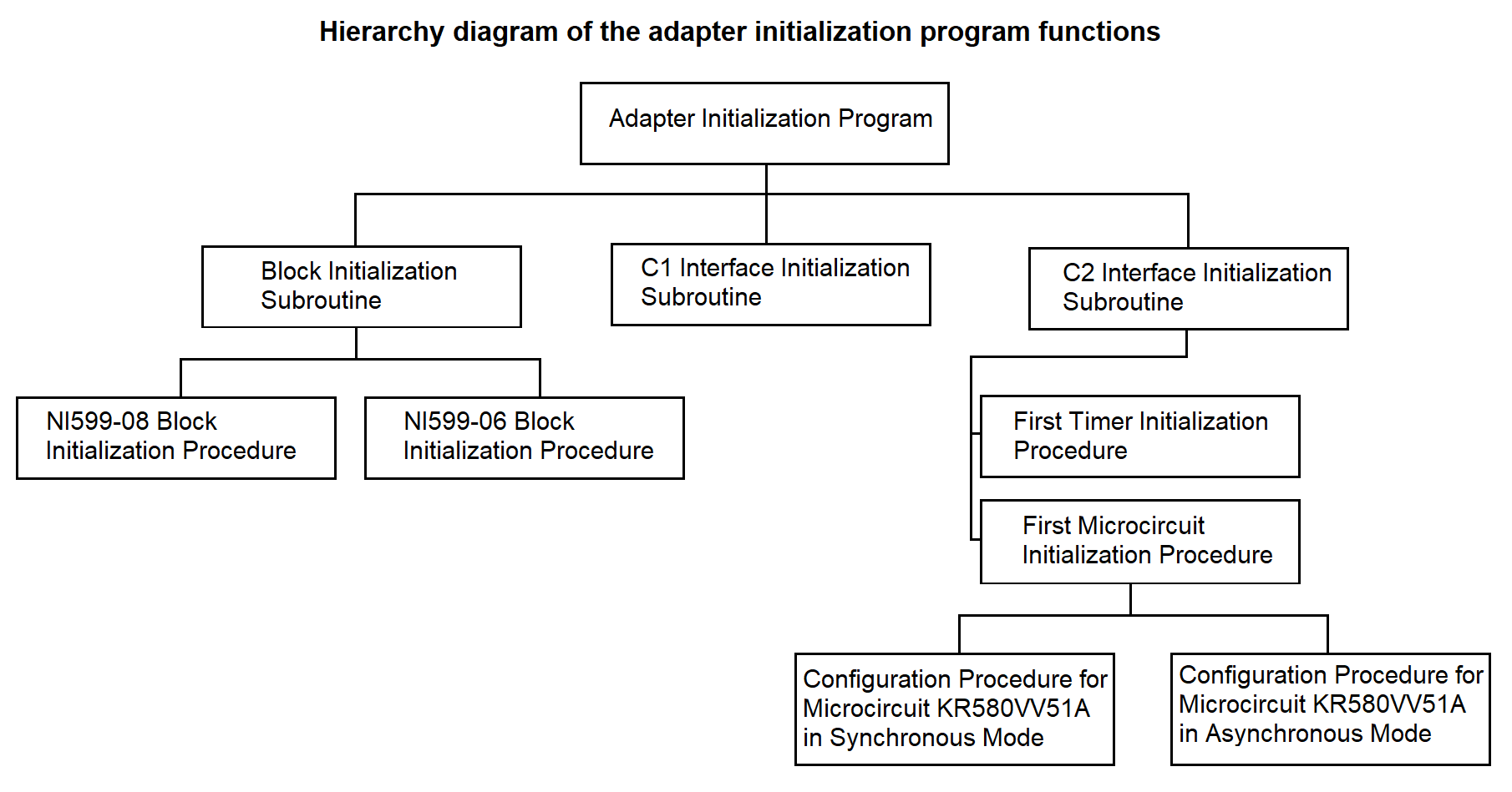
Figure 3.61

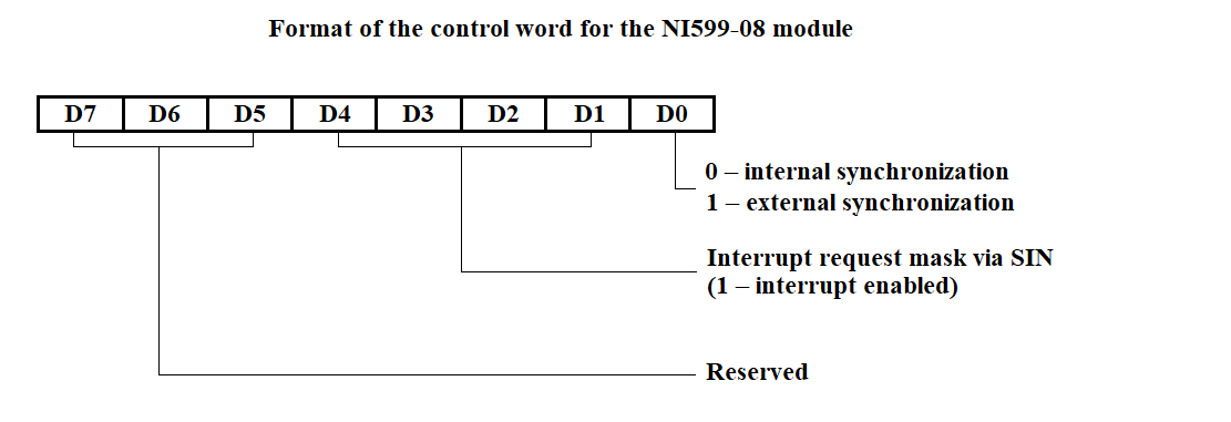
Figure 3.62

The programmable timer is implemented as three independent 16-bit channels with a common control scheme. Programming of channel operating modes is performed individually by entering control words (CW) into the channel mode registers, and counter constants into the counters. The constant is set depending on the data reception or transmission rate in accordance with Table 3. The format of the timer control word is shown in Figure 3.63.

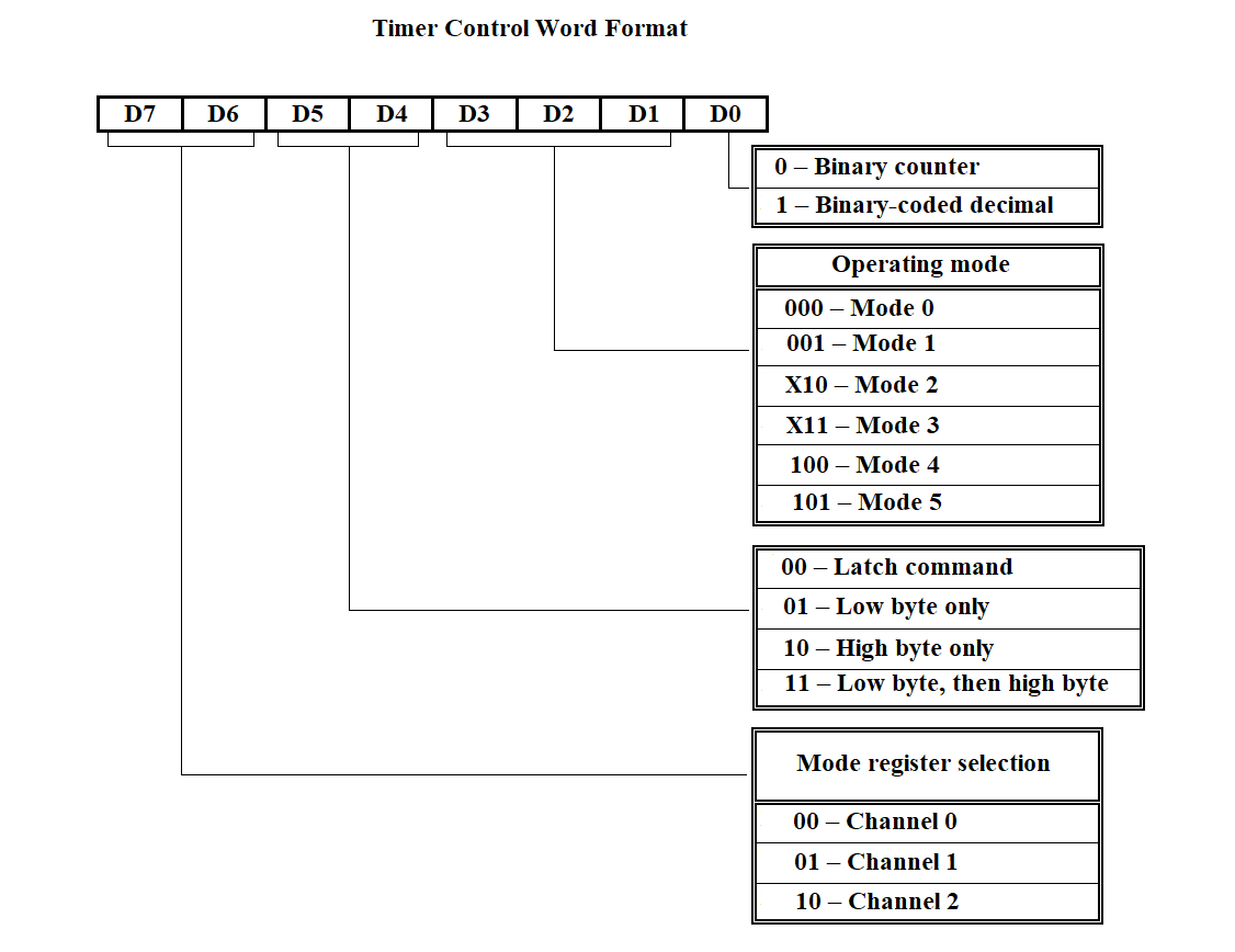
Figure 3.63

The USART (Universal Synchronous/Asynchronous Receiver/Transmitter) operates in two modes: synchronous and asynchronous. Programming the microcircuit for either mode is performed by writing to the appropriate registers: the mode instruction register, sync character register (for synchronous mode), and command instruction register. The format of the mode instructions for both synchronous and asynchronous operation is shown in Figure 3.64. The format of the command instruction is shown in Table 4. I/O port addresses and the configured operating modes of the NI599-06 module are provided in Table 5.

Table 4

Command Instruction Format

Table 5

I/O Port Addresses of Module NI599-08

XX — Group address of the module

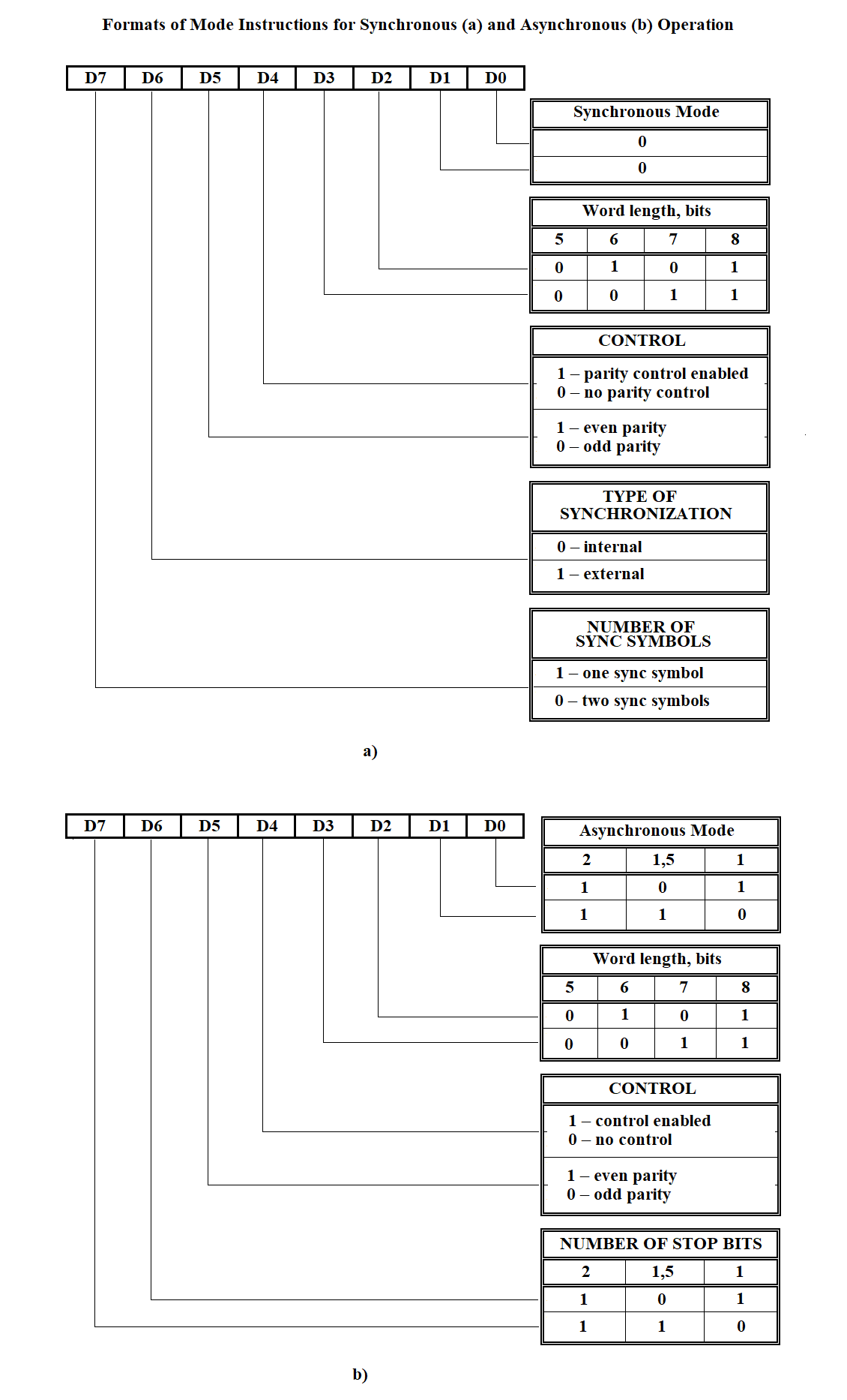
Figure 3.64

ADAPTER INITIALIZATION PROGRAM

The block initialization subroutine is running
Channel number CN := 1

LOOP-WHILE CN is less than or equal to the total number of channels
In the processor configuration table at address =
= table address + (CN - 1) * 66H + 28H, take the chip address (2 bytes)
In the processor configuration table at address =
= table address + (CN - 1) * 66H + 48H, take the adapter type (4 bits)
IF adapter type = 0010B   /* adapter of type C2 */
Run the initialization subroutine for connector C2
ELSE run the initialization subroutine for connector C1
END-IF
CN := CN + 1
END-LOOP
    

BLOCK INITIALIZATION SUBROUTINE

Channel number CN := 1

LOOP-WHILE CN ≤ total number of channels
In the processor configuration table at address =
= table address + (CN - 1) * 66H + 28H, take the chip address (2 bytes)
Clear the lower byte of the chip address   /* determine the block’s own address */

IF in the Register of Initialized Blocks (RIB),
the bit corresponding to channel CN is NOT set to 0
In the processor configuration table at address =
= table address + (CN - 1) * 66H + 48H, take the adapter type (4 bits)
IF adapter type = 0010B   /* adapter of type C2 */
run initialization procedure for block NI599-08
ELSE   /* adapter of type C1 */
run initialization procedure for block NI599-06
END-IF
END-IF

CN := CN + 1
Set bit CN in RIB to 1

END-LOOP
    

BLOCK INITIALIZATION PROCEDURE NI599-08

Channel number CN := 1
WHILE CN ≤ total number of channels
In the processor configuration table at address =
table address + (CN - 1) * 68H + 28H
retrieve the chip address (2 bytes long)

In the processor configuration table at address =
table address + (CN - 1) * 68H + 4CH
retrieve the adapter operation mode (2 bytes long)

IF operation mode = 00   /* synchronous */
Determine the block number BN1 using the chip address

IF BN = BN1   /* block is the same */
Select the lower byte of the chip address
CASE 12H:
BCW := BCW 00000010B   /* BCW - Block Control Word */
CASE 1AH:
BCW := BCW 00000100B
CASE 22H:
BCW := BCW 00001000B
CASE 2AH:
BCW := BCW 00010000B
END CASE
END IF
END IF

CN := CN + 1
END WHILE

Write the control word BCW to the block using its own address and BN number
    

INITIALIZATION SUBROUTINE FOR CONNECTOR C2 (RS-232 INTERFACE)

Clear the lower byte of the microcircuit address   /* determine the block’s
 own address */
The first timer initialization procedure is running.
The first microcircuit initialization procedure is running.
    

FIRST TIMER INITIALIZATION PROCEDURE

From the processor configuration table at address = table address + (CN-1)*68H + 20H  
retrieve the counter constant (1 byte);  
SELECT lower byte of chip address  
CASE 12H  
CCW := 00101111  /* Counter Control Word */  
Send CCW to address = module base address + 000EH  
Send lower byte of counter constant to address =  
module base address + 0008H  

CASE 1AH  
CCW := 01001111  
Send CCW to address = module base address + 0006H  
Send lower byte of counter constant to address =  
module base address + 0002H  

CASE 22H  
CCW := 10101111  
Send CCW to address = module base address + 0006H  
Send lower byte of counter constant to address =  
module base address + 0004H  

CASE 2AH  
CCW := 00101111  
Send CCW to address = module base address + 0006H  
Send lower byte of counter constant to address =  
module base address  

END SELECT
    

FIRST SUBROUTINE FOR INITIALIZING THE MICROCHIP

In the processor configuration table at the address = table address + (CN-1)*68H +
4CH retrieve data on the microchip operating mode (synchronous, asynchronous)
with a length of two bits;
IF operating mode = 00B   /* synchronous */
Execute the routine for configuring the KR580VV51A microchip to synchronous
operating mode;
ELSE   /* asynchronous */
Execute the routine for configuring the KR580VV51A microchip to synchronous
operating mode;
END-IF

FIRST PROCEDURE FOR INITIALIZING MICROCHIP KP580BB51A FOR SYNCHRONOUS MODE

Mode Instruction (MI) := 00010000B  
/* synchronization type — internal, control enabled (even or odd parity) */

From the PROCESSOR CONFIGURATION TABLE, get the data on the number of sync symbols  
at address = table address + (CH–1)*68H + 52H, 2 bytes long,  
the type of control from address = table address + (CH–1)*68H + 50H, 2 bytes long,  
the byte length from address = table address + (CH–1)*68H + 4EH, 2 bytes long

IF byte length = 11B   /* 8 → D2 = 1 and D3 = 1 */  
MI := MI + 00001100B  
END-IF

IF control type = 11B   /* parity control */  
MI := MI + 00100000B  
END-IF

IF number of sync symbols = 01B   /* one sync symbol */  
MI := MI + 10000000B

Send Mode Instruction (MI) to microchip address
From the PROCESSOR CONFIGURATION TABLE, at address =
table address + (CH–1)*68H + 58H, get the first sync symbol, 1 byte long
Send the sync symbol to microchip address
Send Command Instruction (CI) := 10110111B to microchip address

ELSE   /* two sync symbols */
Send Mode Instruction (MI) to microchip address
From the PROCESSOR CONFIGURATION TABLE, at address =
table address + (CH–1)*68H + 58H, get the first sync symbol, 1 byte long
Send the first sync symbol to microchip address
From the PROCESSOR CONFIGURATION TABLE, at address =
table address + (CH–1)*68H + 60H, get the second sync symbol, 1 byte long
Send the second sync symbol to microchip address
END-IF

Send Command Instruction (CI) := 10110111B to microchip address
    

SUBROUTINE FOR CONFIGURING THE KP580VV51A MICROCHIP FOR ASYNCHRONOUS MODE

Mode Instruction (MI) := 00010000B /* parity control enabled, 1:16 operating mode */

From the PROCESSOR CONFIGURATION TABLE, retrieve:
stop bit length  
from address = table address + (CN–1)*68H + 56H, 2 bits long
control type  
from address = table address + (CN–1)*68H + 50H, 2 bits long
byte length  
from address = table address + (CN–1)*68H + 4EH, 2 bits long

IF stop bit length = 11B   /* two stop bits */  
MI := MI + 11000000B  
END-IF

IF control type = 11B   /* parity control */  
MI := MI + 00100000B  
END-IF

IF byte length = 11B   /* 8 bits → D2 = 1 and D3 = 1 */  
MI := MI + 00001100B  
END-IF

Send Mode Instruction (MI) to microchip address  
Send Command Instruction (CI) := 10110111B to microchip address
    

3.4.5. Data Entry Program for RC Configuration

The program is intended for creating and modifying the configuration file of the Remote Concentrator (RC). The file stores multiplexer line numbers and IP types. For the file structure, see section 3.3.7.

The hierarchy diagram of the data entry program functions for RC configuration is shown in Figure 3.73.

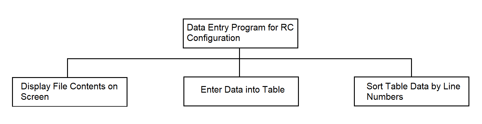
Figure 3.73

Configuration Data Entry Program in Pseudocode in Figure 3.74.

Open file
IF file does not exist
Create file
Open file
END-IF
Display file contents on screen
IF you want to enter new data or modify existing ones
WHILE requests are received
Enter multiplexer line number
IF such number exists
Enter new IP type
END-IF
Enter IP type value
END-WHILE
END-IF
Close file
    

3.4.6.Program for generating the configuration tables of the processor

The program is intended for creating and modifying the processor configuration table, which is then loaded into the SP. The program receives input data entered from the keyboard in response to prompts.

The output data is a file.

The file structure is presented in section 3.3.7.

The function hierarchy diagram of the program for configuring external links of the SP is shown in Figure 3.75.

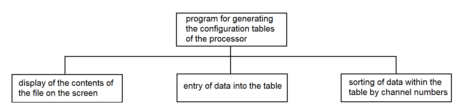
Figure 3.75

Программа формирования таблиц конфигурации процессора на рис. 3.76.

Program for generating the configuration tables of the processor in Figure 3.76.

Open file
IF file does not exist
Create file
Open file
END-IF

Display file contents on screen

IF you want to modify the table
IF you want to fill a new row in the table
WHILE there are input requests
Enter channel number
WHILE number of columns in the table <= number of input values
Enter remaining data, separating them by pressing the "Enter" key
END-WHILE
END-WHILE
END-IF

IF you want to modify individual data in any row
Specify channel number
Make changes in the required column
END-IF
END-IF

Close file
    

3.4.7.Program for Generating the File of the Initialization Segment of Interrupt Vectors

The program is intended for creating and modifying the interrupt vector initialization segment file. The file stores the numbers of new interrupt vectors and the addresses of interrupt handler programs, and also maps new handler addresses to existing interrupt vector codes.

The input data of the program are the interrupt vector numbers and the addresses of interrupt handler programs, entered from the PC keyboard. The output is the interrupt vector initialization segment file intended for loading into the SP.

Structure of the file is provided in Section 3.3.7.

The hierarchy diagram of the interrupt vector initialization segment file generation program is shown in Figure 3.77.

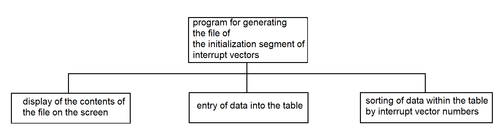
Figure 3.77

Program for Generating the File of the Interrupt Vector Initialization Segment In pseudocode in Figure 3.78.

Open the file
IF the file does not exist
Create the file
Open the file
END-IF

Display the contents of the file on the screen

IF you want to enter new data and modify existing data
WHILE input requests are coming
Enter the vector number
IF such a number exists
IF you want to continue
Enter a new value for the interrupt handler address
END-IF
END-IF
Enter the value of the interrupt handler address
END-WHILE
END-IF

Close the file
    

3.4.8. Program for Generating the SP Load Segment File

The program prepares the SP load segment file, which is then used by the loading program. The loading program loads data into the Synchronization Processor (SP) using the information stored in the segment file. See the structure of the file in p. 3.3.7. Each line of the segment file contains information about a data segment that should be loaded into the SP. This information is entered during the program’s dialog with the operator. The output data of the program is the SP load segment file.

The function hierarchy of the SP load segment file generation program is shown in Figure 3.79.

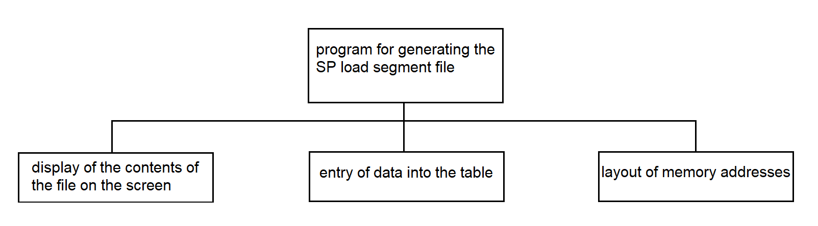
Figure 3.79

Program for Generating the SP Load Segment File in pseudocode in Figure 3.80.

Open file
IF file does not exist
                Create file
                Open file
END-IF

Display contents of the file on the screen

IF you wish to modify the table
Count the number of rows in the table N
WHILE requests are received
Enter segment name
Calculate segment length
IF segment name already exists
Clear the value in the segment length column of the current row
Enter the new segment length value
END-IF
Write the segment length value into the table DS(N)
Determine the new segment number N++
Write N into the segment number column of the current row
END-WHILE

IF memory address planning is automatic
Assign address AD(1) = 1000 to segment number N(1)
WHILE row number N(N) <= number of rows in table N
Assign the address to segment N(N), calculated as the sum of 
segment length DS(N–1) and the corresponding address AD(N–1) of
 the previous row in the table
END-WHILE
END-IF

Enter address values in descending order of segment numbers,
separating them with the "Enter" key
END-IF

Close file
    

3.4.9. Continuous Testing Program of the SP from the PC Side

The program is intended to control the functioning of the multiplexer and the Synchronization Processor (SP), as well as to check the operability of both processors of the synchronization system.
The program outputs a file that logs the time of error occurrences.
The file structure is described in section 3.3.7.

The program performs the following functions:

1. Send a byte to the channel.
2. Receive a byte from the channel.
3. Compare the two bytes. If they match, the program continues operating; otherwise, it logs an error in the log file.

The byte is sent periodically, approximately every 10–60 seconds.

The continuous testing program uses system calls:

1. ALARM – set an alarm for the process;
2. SIGNAL – specify actions for signal handling;

The following library functions are used:

1. FOPEN – open a stream;
2. FREAD, FWRITE – binary input/output;
3. FSEEK – set stream position;
4. PRINTF – formatted output;
5. GETCHAR – read a character or word from the stream.

The function hierarchy diagram of the continuous testing program from the PC side is shown in Figure 3.81.

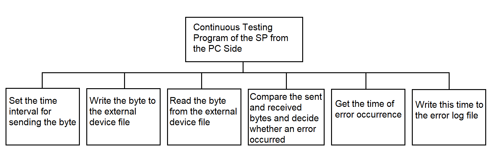
Figure 3.81

Continuous Testing Program in Pseudocode in Figure 3.82.

Open the file of the external device
Open the error log file

WHILE the interrupt signal from the timer is received
Set the byte sending time interval
Write the byte to the external device file
Read the byte from the external device file
Compare the sent and received bytes
IF the bytes are not equal
Get the time of the error occurrence
Write this time to the error log file
END-IF
END-WHILE
    

3.4.10. Program for Continuous Testing of the SP from Processor 1

The continuous testing program from Processor 1 is intended to control the operation of a multiplexer of the MULTISERIAL type and the SP. The program operates in conjunction with the continuous testing programs of the SP from Processor 2 and the PC. Testing data is sent to the SP and received from the SP by the PC-side continuous testing program. When a data byte is received from the communication line, the program writes it to a buffer using the standard buffer write procedure located in the shared memory area.

The functional hierarchy diagram is shown in Figure 3.83.

Figure 3.83

Program for Continuous Testing of the SP from Processor 1 — see Figure 3.84.

READ data byte from microchip
WRITE byte to buffer
    

3.4.11. Continuous Testing Program of the SP from Processor 2

The program operates in the SP. The continuous testing program from processor 2 is designed to control the operation of the MULTISERIAL multiplexer and the SP. The program works in conjunction with the continuous testing programs of the SP from processor 1 and the PC.

The hierarchy diagram is shown in Figure 3.85.

Figure 3.85

Continuous Testing Program of the SP from Processor 2, see Figure 3.86.

READ a byte from the buffer
TRANSMIT the data byte
    

Procedure: read a byte from the buffer in Figure 3.87.

Load the BX register with the value: channel number * 100 – 100 [+50]
IF BOX[BX + 3] > 0
Take the value from cell BOX[BX + 2] and load it into SI
Read the byte of information at address BOX[BX + SI]
Increment BOX[BX + 1] by 1

IF BOX[BX + 3] = 1
Clear the low byte in BOX[BX]
END-IF

Decrement BOX[BX + 3] by 1
END-IF
    

3.4.12. Interrupt Identification Program by Processor 1

The program operates in the SP. It starts working upon hardware interrupt control transfer for receiving information from the communication line. Upon receiving control, it polls the Status Command Register (SCR) of the involved adapters, and upon detecting the channel through which the information arrived, generates a software interrupt to the program servicing that channel.

SCR addresses are calculated via offsets to the addresses of the involved microcircuits. The addresses of each channel’s microcircuits are stored in the processor configuration table. In the configuration table, unused adapter address fields contain a zero value, which allows distinguishing fields that contain information from empty fields.

The function hierarchy diagram is shown in Figure 3.88.

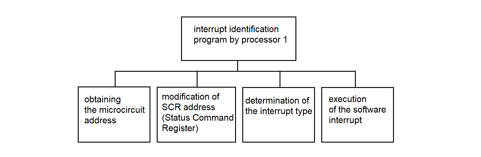
Figure 3.88

Interrupt identification program by processor 1 in Figure 3.89.

Get the microcircuit address
Modify the adapter address to the RCS address
At the RCS address, check the presence-of-data flag
IF data is present
Retrieve the interrupt type for reception 
             from the configuration table of processor 1
Execute a software interrupt
END-IF
    

3.4.13. Interrupt Identification Program for Processor 2

The interrupt identification program for processor 2 is analogous to the interrupt identification program for processor 1.

3.4.14. Data Reception Driver from MS "Vega"

The data reception driver from "Vega" operates in the SP. It is intended for receiving data bytes from the synchronous communication line between the RC and the MS "Vega". The driver receives data in two modes: transparent and non-transparent. In transparent mode, the odd-numbered DLE character is removed, as well as the padding characters DLE and SYN. In non-transparent mode, the SYN padding characters are removed.

The hierarchy diagram of the driver is shown in Figure 3.90.

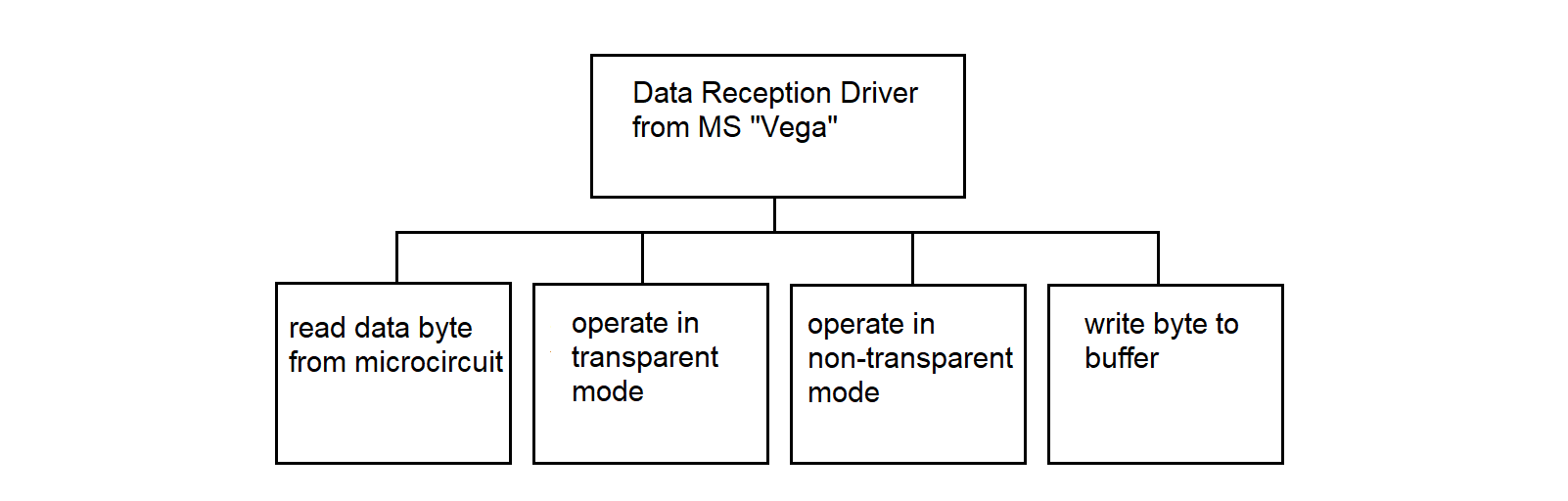
Figure 3.90

Data reception driver from "Vega" in Figure 3.91.

read a data byte from the line;
if the transparent mode bit is set
    operate in transparent mode;
else
    operate in non-transparent mode;
end-if
    

Procedure for Operation in Transparent Mode, see Figure 3.92.

IF the DLE bit is cleared
IF the data byte is DLE THEN
Set the DLE bit;
ELSE
Write the byte to the buffer;
ENDIF
ELSE   /* i.e., if the DLE bit is set */
IF the data byte is one of ETX, ETB, US, ENQ THEN
Clear the transparent mode bit;
Write DLE to the buffer;
Write the byte to the buffer;
Clear the DLE bit;
ENDIF
IF the data byte is SYN THEN
Clear the DLE bit;
ENDIF
IF the data byte is DLE THEN
Write DLE to the buffer;
Write the byte to the buffer;   /* second DLE */
Clear the DLE bit;
ENDIF
ENDIF
    

Procedure for operating in non-transparent mode, see Figure 3.93.

IF bit DLE is set THEN
IF data byte is STX THEN
Write DLE to buffer;
Write STX to buffer;
Set transparent mode bit;
ELSE
Write DLE to buffer;
Write byte to buffer;
ENDIF
ELSE   /* bit DLE is not set */
IF data byte is SYN THEN
Transmit nothing;
ENDIF
ENDIF
    

Byte Buffer Write Procedure Figure 3.94.

/* BOX is the label for the start of the mailbox area */

Load into register BX the value: channel number * 100 – 100 [+50]
IF BOX[BX + 3] > 0 THEN
Retrieve the value from cell BOX[BX + 2] and send to SI
Write the data byte at address BOX[BX + SI]
Increment BOX[BX + 2] by 1
Increment BOX[BX + 3] by 1
Set the data-available bit in the status byte
END-IF
    

3.4.15. Driver for Receiving Data from MS "Kama"

The data reception driver from the "Kama-A" system (hereinafter referred to as "Kama") is intended for receiving information from the MS "Kama", assigning a subchannel number to the data, and writing the information into the mailbox (MB).

The development of this program is based on the following features and conventions:

• The maximum data reception rate from "Kama" is 200 baud;
• The number of data bits in a byte from "Kama" is 5;
• The data arriving at the SP from multiple telegraph lines is multiplexed and transmitted to the PC via a single line of connector C2;
• The transfer to the PC is performed using 8-bit transmissions, of which three bits are used to identify the telegraph channel number;
• Reading from the line and writing to the buffer is done using standard procedures.

The driver hierarchy diagram is shown in Figure 3.95.

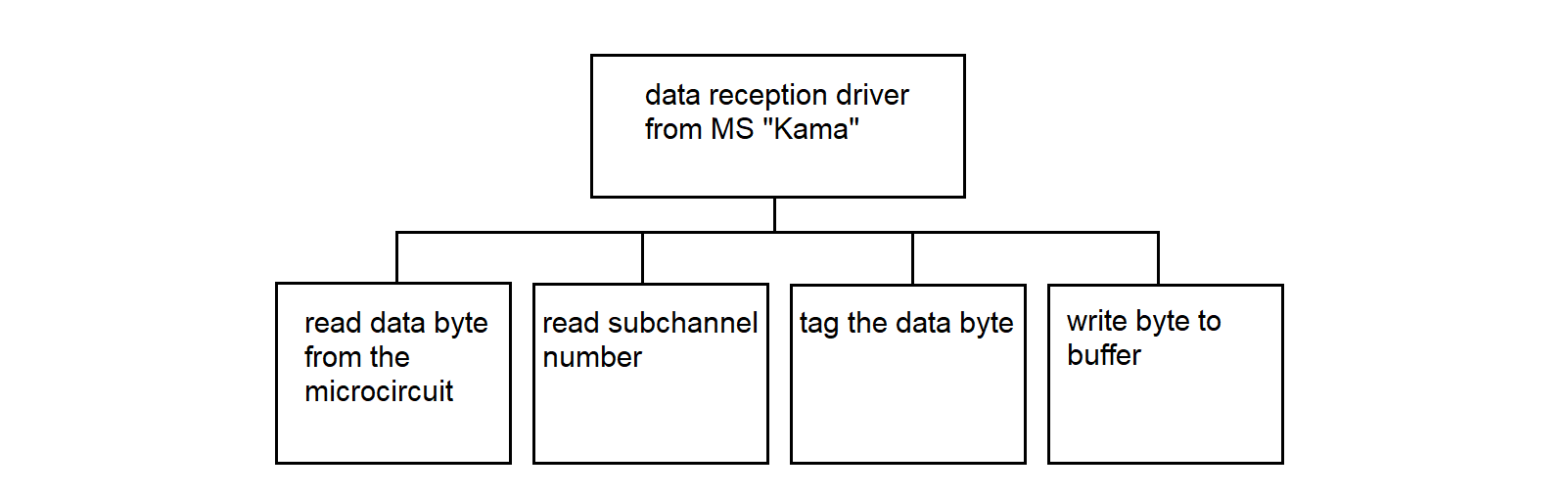
Figure 3.95

Data Reception Driver from "Kama" Figure 3.96.

Read data byte from the microcircuit
Read subchannel number
Mark the data byte
Write the byte to the buffer
    

3.4.16. Data Reception Driver from the PC to MS "Vega"

The data reception driver from the PC to "Vega" operates in the SP. The driver receives data bytes according to the interaction protocol with "Vega" (see section 3.3.3). The driver writes data bytes to the buffer and sets flags, allowing the data transmission program to "Vega" to track continuous character sequences (GOST 28079–89).

The hierarchy diagram of the driver is shown in Figure 3.97.

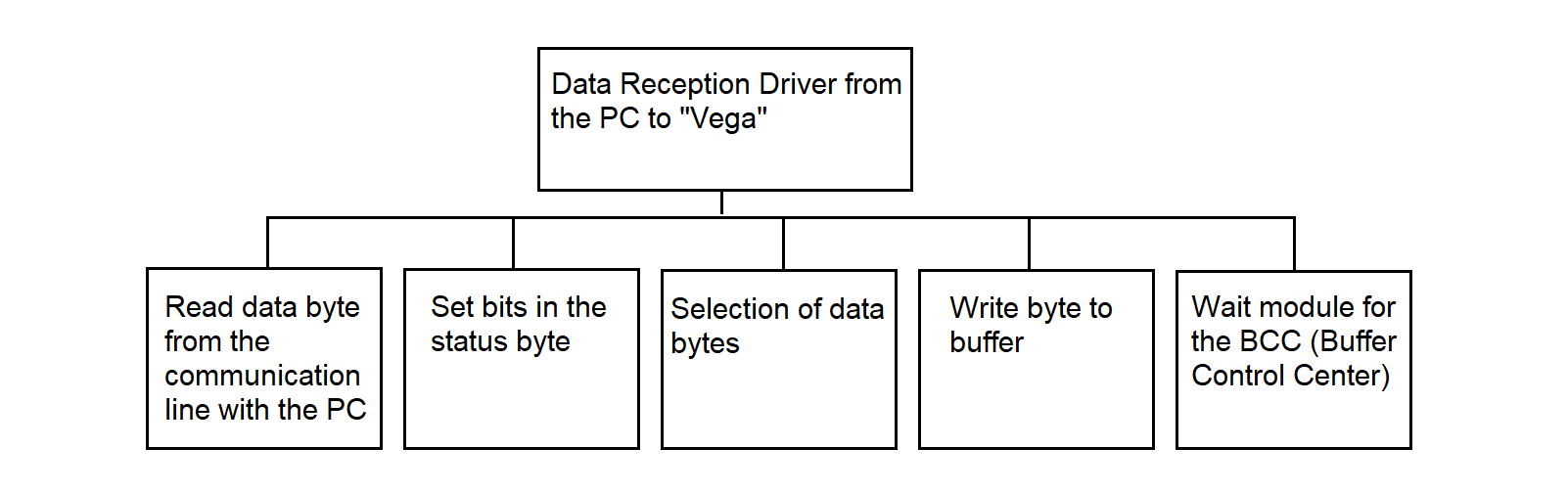
Figure 3.97

Data reception driver from the PC to "Vega", Figure 3.98.

Read a data byte from the communication line to the PC

IF the BCC wait bit is set
Execute the BCC wait module
ELSE
IF the DLE bit is cleared
IF the data byte is DLE
Write to cell 4 from cell 2
Set the transmission inhibit bit
Write the byte to buffer
Set the DLE bit
ELSE  /* writing a text (information) byte */
Write the byte to buffer
Write to cell 4 from cell 2
END-IF
ELSE  /* i.e., if the DLE bit is set */
SELECT the data byte
CASE DLE:
Write the byte to buffer
Write to cell 4 from cell 2
Clear the transmission inhibit bit
Clear the DLE bit
CASE ETX or ETB or US:
Write the byte to buffer
Clear the DLE bit
Clear the transparent mode bit
Set the BCC wait bit
CASE STX:
Clear the transmission inhibit bit
Write the byte to buffer
Write to cell 4 from cell 2
Clear the DLE bit
Set the transparent mode bit
DEFAULT:
Clear the transmission inhibit bit
Write the byte to buffer
Write to cell 4 from cell 2
Clear the DLE bit
END-SELECT
END-IF
END-IF
    

BCC Waiting Module Figure 3.99.

IF the bit of the 1st BCC byte is set THEN
Write byte to buffer
Copy contents of cell 2 to cell 4
Clear the transmission prohibition bit
Clear the DLE bit
Clear the BCC waiting bit
Clear the bit of the 1st BCC byte
ELSE
Write byte to buffer
Set the bit of the 1st BCC byte
END-IF
    

The status byte in the mailbox section when passing information from the PC to "Vega" is shown in Figure 3.100. The digits indicate the bits of the status byte.

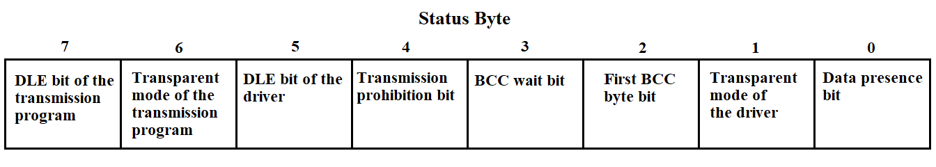
Figure 3.100

3.4.17. Mailbox Scanning Programs

The program checks for the presence of data in the mailbox, transferred from one SP to another, and passes the data to the processing program.

The program must check the information presence bit in the status byte located in the 50-byte section of the mailbox. When the presence bit is set, the scanning program refers to the processor configuration table and performs a software interrupt to the data transfer program.

The mailbox scanning program in pseudocode is shown in Figure 3.101.

WHILE the channel exists in the processor table
Find the address of the second 50-byte section of the mailbox
Check the information availability bit
IF the bit is set THEN
Using the channel number, find the microcircuit address
Using the microcircuit address, find the Status Command Register (SCR)
Check readiness for transmission
IF ready THEN
Determine the type of interrupt for transmission
Execute software interrupt
END-IF
END-IF
END WHILE
    

The information scanning program in the Synchronization Processor by processor 2 differs from the information scanning program by processor 1 in that the first 50-byte section of each mailbox involved in the data exchange is scanned.

3.4.18. Data Transmission Program to MS "Vega" from PC

The information transmission program from the PC to "Vega" performs transmission in accordance with the exchange protocol with "Vega". The program operates in the Interface Processor (IP). It transmits data bytes from the Mailbox (MB) to the Measuring System (MS). The program gains control via a software interrupt from the MB scanning program. The algorithm allows uninterrupted transmission of sequences DLE ETB, (DLE ETX, DLE US), BCC, and DLE DLE, which prevents insertion of padding characters into these sequences. The hierarchy diagram of the program is shown in Figure 3.102.

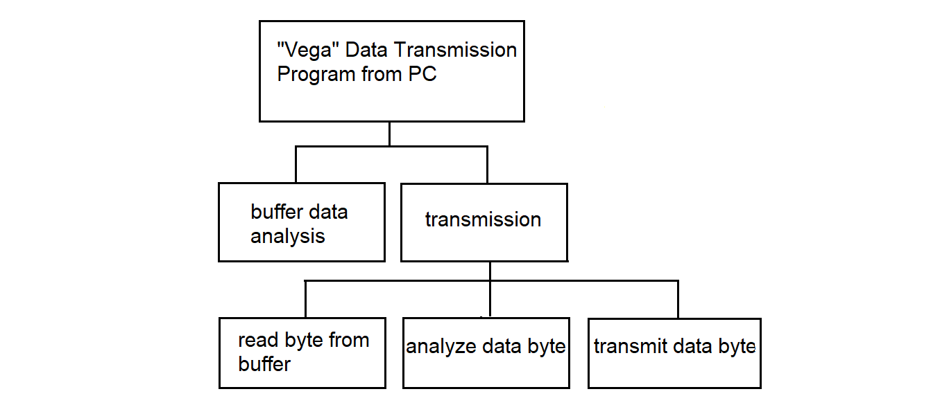
Figure 3.102

Read byte from cell 4 of the mailbox
Read byte from cell 1 of the mailbox

IF byte from cell 4 ≠ byte from cell 1
Transmit
END-IF

IF byte from cell 4 = byte from cell 1
IF transmission lock bit is cleared
Transmit
END-IF
END-IF
    

In the data transmission program to "Vega" from the PC, the procedure "Transmission" is used — see Figure 3.104.

Procedure: Transmission

Read byte from buffer
IF DLE bit is set THEN
IF data byte is STX THEN
Transmit data byte
Enable transparent mode
Clear DLE bit
END-IF
IF data byte is ETX or ETB or US THEN
Transmit data byte
Disable transparent mode
Clear DLE bit
END-IF
ELSE
Transmit data byte
END-IF
    

3.4.19. Data Transmission Program to the PC from MS "Vega"

The data transmission program to the PC from MS "Vega" operates in SP. The program receives control from the mailbox scanning program through a software interrupt. When a circular buffer is used to store information in the MB for all channels, regardless of the type and nature of the information, unified reading and writing to the buffer are applied. The functional hierarchy diagram of the data transmission program to the PC from "Vega" is shown in Figure 3.105.

Figure 3.105

Read byte from buffer
Transmit data byte
    

3.4.20. Data Transmission Program from MS "Kama" to PC

The information transmission program from "Kama" to the PC operates in the Synchronization Processor (SP). When using a ring buffer to store information in the Mailbox (MB) for all channels, regardless of the type and nature of the information, a unified read and write to the buffer is used. The functional hierarchy diagram of the information transmission program from "Kama" to the PC is shown in Figure 3.107.

Figure 3.107

Information Transmission Program to PC from "Vega" Figure 3.106

3.4.21. Dispatcher Program

The dispatcher program loads and starts parallel processes, one process per MS. Each process receives information from the SP, forms messages from the incoming byte stream, saves the received messages in the file system of the RC, and sends these messages to the network.

The input data for the dispatcher program is the information contained in the “MP CONFIGURATION” file.

The result of the dispatcher program's operation is a set of parallel processes for receiving, storing, and transferring information from MS to the Data Center (DC), see Figure 3.109.

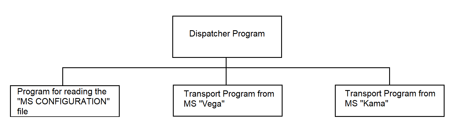
Figure 3.109

The dispatcher program launches the program for reading the "MP CONFIGURATION" file. As a result of executing the file reading program, the "MP CONFIGURATION" array is filled. The dispatcher program iterates through all elements of the "MP CONFIGURATION" array and, based on the channel associated with the MS, launches the corresponding process.

The dispatcher program uses the following programs:

• Reading the "MP CONFIGURATION" file;
• Transport from MS "Vega";
• Transport from MS "Kama".

The composition and number of used programs may vary.
Dispatcher program in pseudocode: Figure 3.110.

Read the file "CONFIGURATION MP" into the array "CONFIGURATION MP"

LOOP — FOR each element of the "CONFIGURATION MP" array
SELECT MS TYPE
CASE 0: No action
CASE 1: Transfer from MS "Vega"
CASE 2: Transfer from MS "Kama"
END SELECT
END LOOP
    

The program for reading the "MP CONFIGURATION" file uses system calls:

• open file;
• read file;
• close file.

Program for reading the "MP CONFIGURATION" file in pseudocode: Figure 3.111.

Open file "MP CONFIGURATION"
Read file "MP CONFIGURATION" into array "MP CONFIGURATION"
Close file "MP CONFIGURATION"
    

The transport program from MS "Vega" organizes the reception of information from MS "Vega", maintaining the appropriate communication protocol, processing the information (determining the type: real-time scale (RTS) data or playback data), storing the information in the file system of the RC, and transmitting the information to the DC. These functions are performed by the programs:

• receiving messages from MS "Vega";
• processing messages from MS "Vega";

These are independent processes spawned by the transport program from MS "Vega". The transport program from MS "Vega" manages interaction between the spawned processes using a software channel through which data exchange occurs.

The transport program from MS "Vega" uses the system call:

• create channel;

and the programs:

• receiving messages from MS "Vega";
• processing messages from MS "Vega".

Figure 3.112

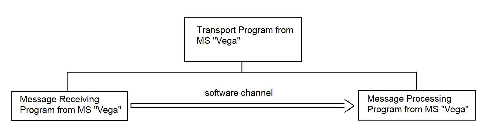
Figure 3.112

The transport program from MS "Vega" in pseudocode is shown in Figure 3.113.

Create channel  
Receive messages from MS "Vega"  
Process messages from MS "Vega"
    

The transport program from MS "Kama" organizes the reception of information coming from MS "Kama" in simplex mode, storage of the information in the file system of the RC, and transmission of the information to the DC. The following functions are performed by the programs:

• receiving messages from MS "Kama";
• processing messages from MS "Kama";

These are independent processes spawned by the transport program from MS "Kama". The transport program from MS "Kama" manages the interaction of the spawned processes through a software channel used for data exchange. Figure 3.114

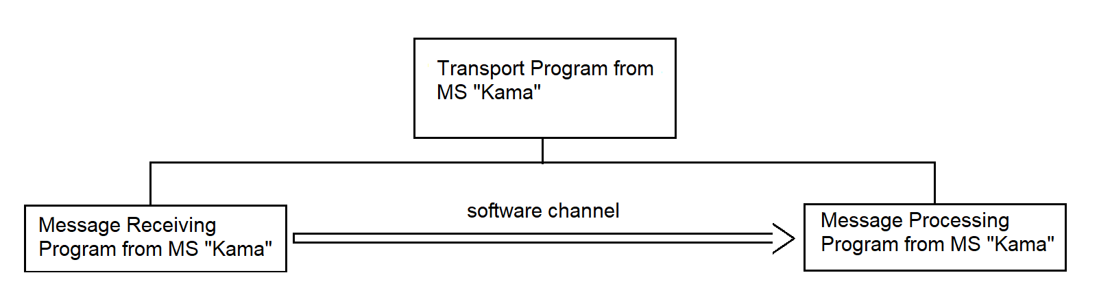
Figure 3.114

The transport program from MS "Kama" uses the system call:

• create channel;

and the programs:

• receiving messages from MS "Kama";
• processing messages from MS "Kama".

The transport program from MS "Kama" in pseudocode is shown in Figure 3.115.

Create channel;
Receive messages from MS "Kama";
Process messages from MS "Kama";
    

3.4.21.1. Message Receiving Program from MS "Vega"

The program is intended for receiving messages from MS "Vega" and transferring them to the communication channel.

At the input, the program receives messages, control sequences (CS), and control characters (CC) coming from the SP. At the output — complete messages sent to the message processing program, as well as control sequences forwarded to the SP.

The program performs the following actions:

1. Supports the BSC communication protocol. Exchange control is carried out using special control characters and control character sequences selected from the permitted set according to GOST 19767-74.

The main exchange procedures are described in section 3.3.3.3.
The structure of the information message received from the SP communication line is shown in Figure 3.116.

Structure of the information message

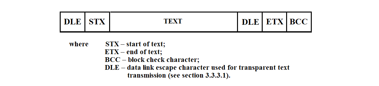
Figure 3.116

2. Receives a message from MS "Vega". Removes control characters (CC), control sequences (CS), and additional symbols (DLE), and passes the message to the processing program.
3. Calculates the block check sequence of the received block and uses the comparison program to verify the correctness of the received information.
   Depending on the comparison results, it issues either a positive or negative acknowledgment for the received message.
4. Analyzes the readiness of the processing program to accept the message and, based on the readiness level, forms a response. Readiness analysis is performed by the readiness and overflow check modules.

The function hierarchy of the message receiving program is shown in Figure 3.117.

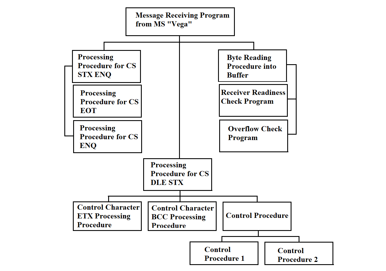
Figure 3.117

After startup, the reception program enters line monitoring mode. Before initiating message transmission, the sending station uses ENQ (Enquiry) to query the receiving station, i.e., RC, for its readiness (establishing logical connection). Upon receiving ENQ, the reception program executes the readiness check procedure (described below) and, if the receiver is ready, generates DLE 0; otherwise — NAK (Negative Acknowledge). After issuing NAK, the program returns to line monitoring mode.

To control the execution flow of the program, the following flags are used:

• End of Transmission Flag (ETF) – is set upon the arrival of DLE STX and characterizes the receive/transmit state; it is cleared upon receiving or sending EOT, which indicates the line monitoring state.

• Format Error Flag (FEF) – is set when an error is detected in the order of control sequences and control characters, or in the structure of the information message during transmission. Setting the FEF causes the program to switch to line monitoring mode. The FEF is cleared upon receiving ENQ.

• DLE0 Flag – is responsible for issuing DLE 0 for each correctly received even block and DLE 1 for each correctly received odd block. It is set upon receiving DLE 0 and cleared upon receiving DLE 1.

• DLE1 Flag – is set upon receiving the first DLE and is cleared upon receiving control characters ENQ, ETB, ETX, or DLE that immediately follow the first DLE 1.

After receiving a connection request from the sending station and issuing a positive acknowledgment, the program is ready to receive data. The End of Transmission Flag (ETF) is cleared. According to the BSC exchange protocol, the main exchange procedures of which are described in section 3.3.3, the reception of the following control sequences and control characters is allowed: EOT, ENQ, STX ENQ, DLE STX. If other control sequences or characters are received, the Format Error Flag (FEF) is set. The program switches to line monitoring mode. To store and process incoming data, the program uses several buffers. The A buffer is used for reading bytes from the communication line. The block buffer (BB) stores the received bytes belonging to one block. The message buffer (MB) accumulates the message text for subsequent transmission to the channel. The check buffer (CB) is used by the verification program. It contains all characters subject to validation. The program pseudocode is provided below.

The message reception program from the "Vega" information system in pseudocode is shown in Figure 3.118.

Operation mode = YES  
Clear End of Transmission Flag (ETF)   /* ETF = 0 */

WHILE operation mode
Execute byte reading routine into buffer A
Reset Byte Counter (BC);   /* BC = 0 */
SELECT content of A:

CASE ENQ        /* who's there? (enquiry) */
Execute ENQ control sequence handler

CASE STX ENQ    /* delay on the sender side */
Execute STX ENQ control sequence handler

CASE EOT        /* end of transmission */
Execute EOT control sequence handler

CASE DLE STX    /* start of text */
Execute DLE STX control character handler

CASE none of the above
Set Format Error Flag (FEF)
/* FEF = 1 */

END SELECT
END WHILE
    

The procedure for processing the ENQ control sequence in pseudocode is shown in Figure  3.119.

IF End of Transmission Flag (ETF) is cleared THEN   /* i.e., ETF = 0 */
Execute receiver readiness check
IF receiver is ready THEN
Send DLE 0
Write DLE 0 to Response Output Buffer (RO)
Set DLE0 Flag       /* DLE0 Flag = 1 */
Set End of Transmission Flag (ETF)   /* ETF = 1 */
ELSE   /* not ready */
Send NAK
ENDIF

ELSE   /* ETF = 1 */
Execute receiver readiness check
IF receiver is ready THEN
Execute overflow control procedure
IF overflow detected THEN
Send DLE
ELSE
Send message from RO
ENDIF
ELSE   /* not ready */
Send EOT
Clear End of Transmission Flag (ETF)   /* ETF = 0 */
ENDIF
ENDIF
    

Upon receiving the ENQ control sequence, if the End of Transmission Flag (ETF) is cleared (i.e., the program is in line monitoring mode), the receiver readiness check is executed. If the response is positive, DLE 0 is sent to the communication line and written to the Response Output Buffer (RO). After that, the DLE0 Flag and the ETF are set. If the readiness check indicates that the receiver is not ready, the program generates a NAK control sequence.

The ENQ control symbol may also arrive in receive–transmit mode. When this happens, the readiness‑check routine is executed. If the system is not ready, the EOT (End Of Transmission) control symbol is generated—signaling the end of the connection—the End Of Transmission Flag (ETF) is cleared, and the program switches to line‑monitoring mode. If the system is ready, the overflow‑control routine is executed (see below). If overflow occurs, the DLE (Data Link Escape) control symbol is generated; otherwise, a message is output from the response buffer.

The pseudocode procedure for handling the STX ENQ control symbol is shown in Figure 3.120.

IF the ETF (End Of Transmission Flag) is set   /* ETF = 1 */
OUTPUT NAK   /* Negative Acknowledge */
ELSE   /* ETF = 0 */
/* no response */
SET the Format Error Flag (FEF = 0)
END IF
    

The Vega information system sends an ENQ control symbol instead of the next data block to signal temporary unavailability for transmission. Upon receiving the ENQ control symbol in receive–transmit mode, the receive routine issues NAK and waits for the continuation of transmission. If the ENQ control symbol arrives in line‑monitoring mode, the Format Error Flag (FEF) is set. No response is given.

The pseudocode procedure for handling the EOT control symbol is shown in Figure 3.121.

IF the ETF (End Of Transmission Flag) is set   /* ETF = 1 */
Clear the ETF flag       /* ETF = 0 */
Send an end-of-transmission message to the terminal
ELSE   /* ETF = 0 */
/* no response */
Set the Format Error Flag       /* FEF = 0 */
END IF
    

The "Vega" information system signals to the program—by sending the EOT control symbol—either the end of transmission or a suspension of transmission. The receive routine handles the EOT symbol by sending an end‑of‑transmission message to the terminal. The End‑Of‑Transmission Flag (ETF) is cleared, after which the program switches to line‑monitoring mode.

The pseudocode procedure for handling the DLE STX control symbol is shown in Figure 3.122.

CLEAR the DLE1 Flag        /* DLE1 Flag = 0 */
IF the ETF (End Of Transmission Flag) is cleared   /* ETF = 0 */
SET the Format Error Flag     /* FEF = 0 */
ELSE   /* ETF = 1 */
EXECUTE the “read byte into buffer A” routine
WHILE (A ≠ ETB AND A ≠ ETX AND A ≠ ENQ AND DLE1 Flag ≠ 1)
WHILE (A ≠ DLE1)
WRITE A to Block Buffer (BB)
WRITE A to Check Buffer (CB)
EXECUTE Control1 procedure
EXECUTE “read byte into buffer A” routine
END WHILE
EXECUTE “read byte into buffer A” routine
IF A = DLE1 THEN
WRITE A to Byte Buffer
WRITE A to Check Buffer (CB)
EXECUTE Control1 procedure
ELSE
CLEAR the DLE1 Flag     /* DLE1 Flag = 0 */
END IF
END WHILE

CASE A OF
ENQ     /* ignore data block */
OUTPUT NAK
ETB     /* end of block */
EXECUTE “handle ETB” procedure
ETX     /* end of text */
EXECUTE “handle ETX” procedure
OTHERWISE
SET the Format Error Flag
CLEAR the DLE1 Flag     /* DLE1 Flag = 0 */
END CASE
END IF
    

The MS “Vega,” by sending the EOT control symbol, signals to the program either the end of transmission or a suspension of transmission. The receive routine handles the EOT symbol by sending an end‑of‑transmission message to the terminal. The End Of Transmission Flag (ETF) is cleared, after which the program switches to line‑monitoring mode.

The pseudocode procedure for handling the ETB control symbol is shown in Figure 3.123.

CLEAR the DLE1 Flag         /* DLE1 Flag = 0 */
WRITE ETB to the Check Buffer     /* ETB = End Of Transmission Block */
EXECUTE the Control1 procedure
EXECUTE the “check receiver readiness” routine
IF the receiver is ready THEN
EXECUTE the Control2 procedure
IF result = 0 THEN
FORWARD the Block Buffer (BB) to the Message Buffer (MB)
EXECUTE the “check overflow” routine
IF no overflow THEN
IF DLE0 Flag = 1 THEN
OUTPUT DLE1      /* send DLE1 control symbol */
SET DLE0 Flag = 0
WRITE DLE1 to the Output Buffer (OB)
ELSE   /* DLE0 Flag = 0 */
OUTPUT DLE0      /* send DLE0 control symbol */
SET DLE0 Flag = 1
WRITE DLE0 to the Output Buffer (OB)
END IF
ELSE   /* overflow exists */
OUTPUT DLE1
IF DLE0 Flag = 1 THEN
SET DLE0 Flag = 0
WRITE DLE1 to the Output Buffer (OB)
ELSE   /* DLE0 Flag = 0 */
SET DLE0 Flag = 1
WRITE DLE0 to the Output Buffer (OB)
END IF
END IF
ELSE   /* message received with error */
WRITE NAK to the Output Buffer (OB)
OUTPUT NAK      /* send Negative Acknowledge */
END IF
ELSE   /* receiver not ready */
OUTPUT EOT       /* send End Of Transmission */
CLEAR the ETF Flag       /* ETF = 0 */
END IF
    

The pseudocode procedure for handling the ETX control symbol is shown in Figure 3.124.

CLEAR the DLE1 Flag          /* DLE1 Flag = 0 */
WRITE ETX to the Check Buffer     /* ETX = End Of Text */
EXECUTE the Control1 procedure
EXECUTE the “check receiver readiness” routine
IF the receiver is ready THEN
EXECUTE the Control2 procedure
IF result = 0 THEN
FORWARD the Block Buffer (BB) to the Message Buffer (MB)
FORWARD the Message Buffer (MB) to the channel
EXECUTE the “check overflow” routine
IF no overflow THEN
IF DLE0 Flag = 1 THEN
OUTPUT DLE1       /* send DLE1 control symbol */
SET DLE0 Flag = 0
WRITE DLE1 to the Output Buffer (OB)
ELSE   /* DLE0 Flag = 0 */
OUTPUT DLE0       /* send DLE0 control symbol */
SET DLE0 Flag = 1
WRITE DLE0 to the Output Buffer (OB)
END IF
ELSE   /* overflow exists */
OUTPUT DLE1
IF DLE0 Flag = 1 THEN
SET DLE0 Flag = 0
WRITE DLE1 to the Output Buffer (OB)
ELSE   /* DLE0 Flag = 0 */
SET DLE0 Flag = 1
WRITE DLE0 to the Output Buffer (OB)
END IF
END IF
ELSE   /* message received with error */
WRITE NAK to the Output Buffer (OB)
OUTPUT NAK       /* send Negative Acknowledge */
END IF
ELSE   /* receiver not ready */
OUTPUT EOT       /* send End Of Transmission */
CLEAR the ETF Flag       /* ETF = 0 */
END IF
    

The STX (Start Of Text) control symbol is sent by the transmitting station at the start of the user’s data text. If the text is divided into blocks, STX is sent at the start of each block. Each subsequent data byte read from the communication line is written simultaneously to the block buffer and the check buffer. If two DLE (Data Link Escape) control symbols are received in succession, one of them is discarded. Writing continues until a control sequence DLE ETB, DLE ETX, or DLE ENQ is received.

If the message to be transmitted is divided into blocks, the transmitting station signals the end of a data block with the ETB control symbol and then sends the BCC control symbol. Upon receiving the DLE ETB control symbol, the receive routine stops writing to the block buffer, writes the ETB symbol into the check buffer, and then invokes the control routine to verify the integrity of the received buffer. If the information is received without errors, it issues either the DLE0 or DLE1 control symbol—depending on the DLE0 Flag—and forwards the block from the block buffer to the message buffer.

The ETX control symbol indicates the end of the information message. If the message is divided into blocks, ETX serves as the end of the last block (in place of ETB). Upon receiving the DLE ETX control symbol, the receive routine—after performing all the actions it would on DLE ETB—forwards the assembled message from the message buffer to the communication channel.

By sending the ENQ control symbol at the end of a data block (in place of ETX or ETB), the MS “Vega” indicates that this block should be disregarded. In response to this control symbol, the receive routine issues NAK.

If a control symbol or sequence not handled above is received, the Format Error Flag is set. The program then switches to line‑monitoring mode.

To support the receive routine, the following programs must be developed:

• a receiver readiness‑check routine;
• an information‑control procedure;
• a routine to read a byte from the communication line into buffer A;
• An overflow‑control routine.

The receive routine uses the following system calls:

ALARM – sets the process alarm.

The receiver readiness‑check routine monitors for a failure message. If such a message is present, it returns 1; otherwise, it returns 0. Readiness is checked each time the receive routine must generate a response under the BSC protocol. If a failure occurs during the communication session, the routine issues the EOT control symbol; if it occurs during the initial poll, it issues the NAK control symbol.

The control procedure is designed to compute the block check character of the received information block (BCC1). It is invoked for each symbol received from the MS “Vega” that is subject to verification. When forming the BCC, a cyclic code with generator polynomial x**16 + x**12 + x**5 + 1 (GOST 17422‑72) is used.

BCC1 computation begins after receipt of the DLE STX control sequence. These control sequences at the start of the block must not be included in the BCC1 computation. In the BCC1 computation process, all characters transmitted after the DLE STX sequence are included, except for the first DLE character in the control sequences DLE ETB, DLE ETX, and DLE DLE.

The computation of BCC1 is performed according to the scheme shown in Figure 3.125.

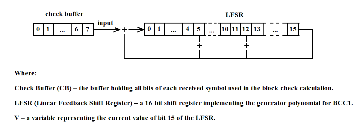
Figure 3.125

BCC1 is computed by performing the following steps:

1. Clear the LFSR.
2. Store the value of bit 15 of the LFSR in V.
3. Shift the contents of the LFSR one bit to the right.
4. Write into the newly vacant bit 0 of the LFSR the value of the last bit of the check buffer (CB), then shift the check buffer one bit to the right.

5. Analyze the value of bit 15 of the LFSR stored in V. If it equals 1, then add 1 modulo 2 to bits 0, 5, and 12 of the LFSR. If V equals 0, no action is required.

Repeat steps 2 through 5 until all information bits from the check buffer (CB) have been sequentially input into the LFSR.

The control2 procedure is designed to verify the correctness of an information block transmission by comparing the BCC1 computed by control1 with the BCC generated by the MS “Vega.” Control2 is invoked by the receive routine each time a block‑receipt acknowledgment must be sent on the communication line. A block is considered error‑free if the check sequences match, and erroneous if they do not.

The byte reading program reads a byte of information from the communication line and places it in buffer A. If the transmission of information from the transmitting station stops, it issues a message to the terminal about the termination of the transmission and switches to line monitoring mode. The program text is given below in Figure 3.126.

IF the Format Error Flag is set   /* FEF = 1 */
Start a timer for n seconds and clear FEF   /* FEF = 0 */
ELSE
Start a timer for n seconds
END IF

WHILE the timer has not expired
Read a byte into buffer A
IF buffer A contains data THEN
RETURN
END IF
END WHILE

OUTPUT a message to the terminal indicating transmission termination  
SWITCH to line-monitoring mode
    

After BCC1 is computed, read 2 bytes from the communication line into BCC2. Compare its contents with the LFSR. If they are equal, return 0 to the receive routine; if not, return 1.

The pseudocode for the control1 procedure is shown in Figure 3.127(a), and for the control2 procedure in Figure 3.127(b).

C = 8      // C – number of bits in the check buffer
WHILE C > 0
STORE the value of bit 15 of the LFSR in V
SHIFT the LFSR one bit to the right
WRITE into bit 0 of the LFSR the value of bit C of the check buffer (CB)
DECREMENT C by 1
IF V = 1 THEN
ADD 1 modulo 2 to bits 0, 5, and 12 of the LFSR
END IF
END WHILE
    

Read 2 bytes into BCC2;   /* BCC2 — buffer holding the received BCC1 */
IF BCC2 = LFSR THEN
RETURN 0    /* no error */
ELSE
RETURN 1    /* message received with error */
END IF
CLEAR LFSR
    

The overflow‑check routine runs each time a positive acknowledgment must be sent on the communication line. It checks whether the receive routine can complete message processing in time. If it can, it returns 0; if not, it returns 1.

3.4.21.2. Message Processing Program from MS "Vega"

The message‑processing program for the Vega measuring system determines the type of incoming information (real‑time data or playback data), stores the received information in the UK’s file system, and forwards it to the programs responsible for delivering it over the network to the collection center.

The input to the Vega message‑processing program consists of messages received via the software channel from the Vega receive routine.

The output of the Vega message‑processing program consists of messages sent over the network using the following primitives:

openpath(), sendviapath(), closepath()

These primitives will be provided by the Scientific and Technical Center of the Plesetsk Cosmodrome.

The diagram of the required functions is shown in Figure 3.128.

The message structure of the Vega system, as well as the message types, are described in section 3.3.1.

Recommendations for naming the storage files for information from the measuring system are provided in section 3.3.7.

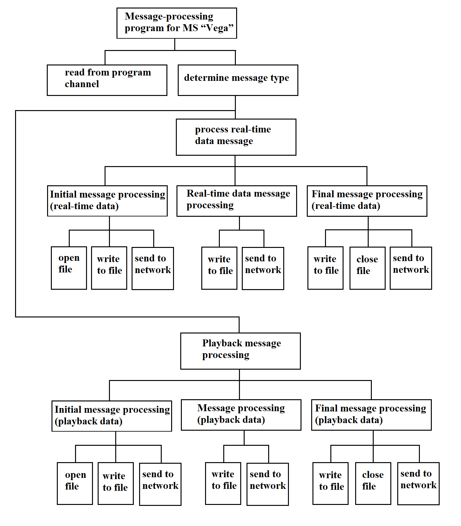
Figure 3.128

The message‑processing program for the “Vega” measuring system is shown in pseudocode in Figure 3.129.

READ the “program channel”
IF information_type = real-time data THEN
SELECT information_index
CASE initial_message
OPEN file
WRITE message to file
SEND message over network
CASE final_message
WRITE message to file
SEND message over network
CLOSE file
CASE message
WRITE message to file
SEND message over network
CASE empty_message
WRITE message to file
SEND message over network
END SELECT
ELSE
SELECT information_index
CASE initial_message
OPEN file
WRITE message to file
SEND message over network
CASE final_message
WRITE message to file
SEND message over network
CLOSE file
CASE message
WRITE message to file
SEND message over network
END SELECT
END IF
    

3.4.21.3. Message Receive Program from MS "Kama"

The message‑receive program for the “Kama” measuring system reads information bytes from the process channel sent by the “Kama” MS, sorts the incoming bytes for each “Kama” MS into its own buffer, and packs the received bytes into a continuous bit stream that constitutes the “Kama” MS information message.

Input: a sequence of bytes arriving from the process channel.

Output: a continuous sequence of bits forming the message, delivered to the program channel for the “Kama” message‑processing routine.

The pseudocode for the “Kama” message‑receive program is shown in Figure 3.130.

READ a byte from the channel  
EXTRACT the three most significant bits  
ms_info := value of those three MSBs   // information from the measuring system

CASE ms_info OF
0: extract message for system 0
…
N: extract message for system N
END CASE
    

The “Extract Message” program in pseudocode is shown in Figure 3.131.

IF byte_value = marker_value THEN
IF marker_flag = TRUE THEN
WRITE message to channel
bit_count := 0
ELSE
bit_count := write byte to packing buffer
marker_flag := TRUE
END IF
ELSE
IF marker_flag = TRUE THEN
bit_count := write byte to packing buffer
END IF
END IF
    

The structure of the message‑receive program for the “Kama” measuring system is shown in Figure 3.132.

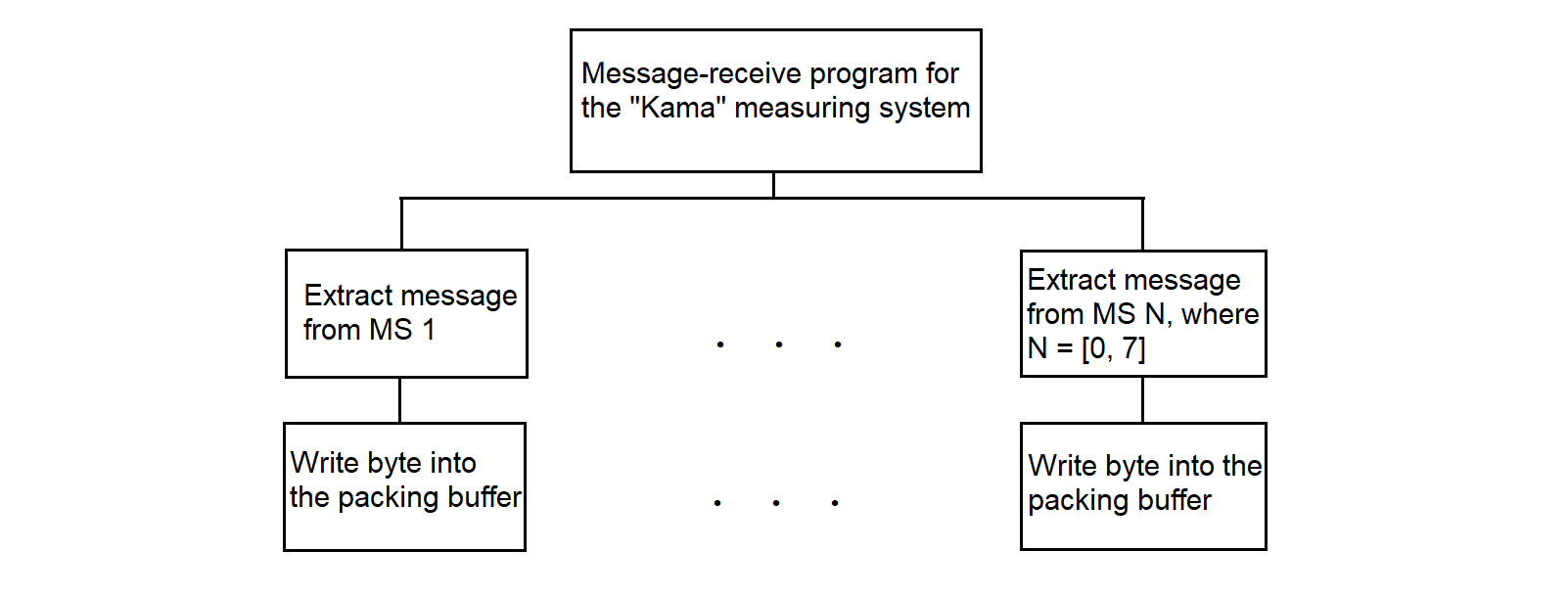
Figure 3.132

The byte‑to‑packing‑buffer routine writes the five least significant bits of each byte received from the “Kama” measuring system into the buffer without gaps, forming a continuous stream of information bits.

The input data for the program for writing a byte into the buffer with packing are 1) the number of bytes written to the buffer, 2) the byte of information from MS, and 3) the buffer address.

The number of bits written into the buffer.

The following abbreviations are used in the pseudocode program description:

• BBA: buffer byte address
• BMS: byte from measurement system
• NBB: number of bits in a byte
• NBW: number of bits written in the MS byte
• NUB: number of unwritten bits in the MS byte
• NMB: number of message bits
• NOB: number of occupied bits in the buffer byte

The program “Write a byte into the buffer with packing” in pseudocode is shown in Figure 3.133.

/* Algorithm for packing telegraph packets into a buffer         */
/* BMS is input byte from measurement system                     */

#define TELEGRAPH_PACKET_SIZE 5   /* Telegraph packet size in bits (from adapter) */
#define NBB 8                     /* Number of bits in one buffer byte         */

BBA := NMB / NBB                 /* Buffer byte address = int(NMB / NBB)       */
NOB := NMB % NBB                 /* Occupied bits in current buffer byte       */
NBW := NMB % NBB                 /* Bits written in MS byte (same as NOB)      */
BMS := BMS << NBW                /* Align new bits with buffer content         */
*BBA := *BBA | BMS               /* Merge BMS with buffer byte at BBA          */
NUB := TELEGRAPH_PACKET_SIZE - NBW  /* Remaining bits of BMS not yet stored    */

IF NUB <= 0 THEN
    NMB := NMB + TELEGRAPH_PACKET_SIZE  /* All 5 bits written in one byte      */
ELSE
    NBW := TELEGRAPH_PACKET_SIZE - NUB  /* Bits written in current byte        */
    NMB := NMB + NBW                    /* Update total bits written           */
    BBA := NMB / NBB                    /* New buffer address                  */
    BMS := BMS >> NUB                   /* Get remaining bits                  */
    *BBA := *BBA | BMS                  /* Merge rest into next buffer byte    */
    NMB := NMB + NUB                    /* Update total bits again             */
END IF

3.4.21.4. Message Processing Program from MS "Kama"

The message processing program for "Kama" MS stores incoming information in the RC file system and forwards it to the CC (collection center).

The input data for the message processing program for "Kama" MS are the messages arriving via the program channel from the "Kama" MS message‑receive routine.

The output data for the message processing program for "Kama" MS are the messages sent over the network using network primitives and those same messages saved in the RC file system.

The message processing program for "Kama" MS organizes transmission of incoming information to the network using the primitives

openpath(), sendviapath(), closepath(),

which will be provided by the Plesetsk Cosmodrome STC (Scientific and Technical Center).

The pseudocode for the message processing program for "Kama" MS is shown in Figure 3.134.

The structure of the message processing program for "Kama" MS is shown in Figure 3.135.

READ "program channel"
SELECT measuring_system_number
CASE 0
OPEN file
WRITE message to file
SEND message over network
CLOSE file
...
CASE 4
OPEN file
WRITE message to file
SEND message over network
CLOSE file
...
END SELECT
    

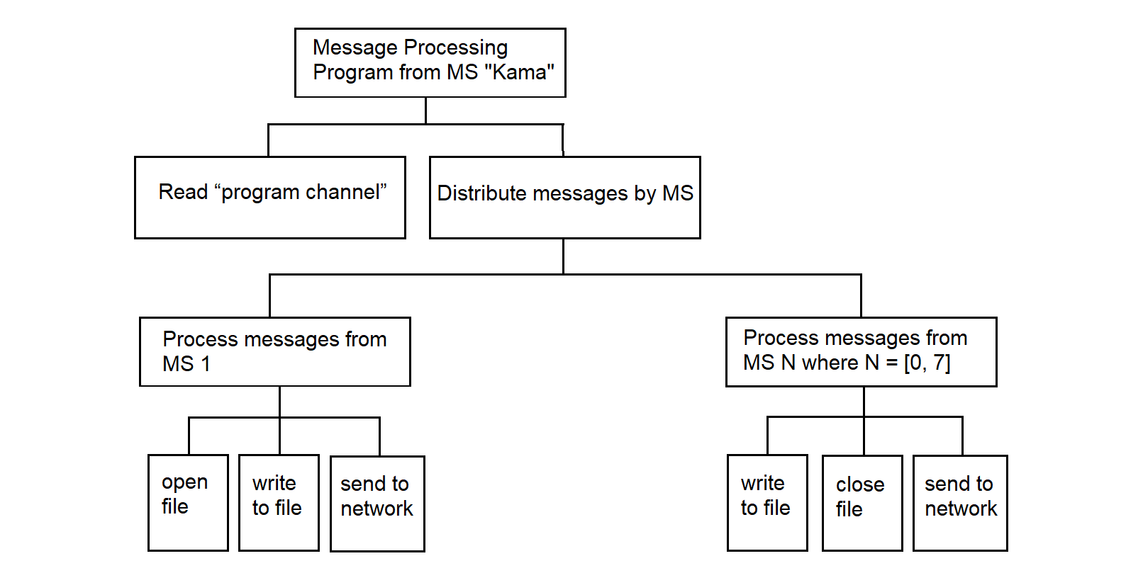
Figure 3.135

3.4.22. Program for Receiving and Distributing Network Information

The network information receive‑and‑distribute program accepts and routes command information from the CC to each MS at each MP, storing it in the RC file system. In addition, it may receive command information from the network for the dispatcher program to launch the required application process.

Input to the receive‑and‑distribute program consists of messages arriving from the network (the structure of these messages is not yet defined, since none of the deployed MS units currently processes incoming network messages—this function is thus implemented as a software stub).

Output from the receive‑and‑distribute program consists of messages sent to specific MS units and saved in the RC file system.

The pseudocode for the receive‑and‑distribute program is shown in Figure 3.136.

RECEIVE message from network
SELECT MS_type
CASE 0
WRITE to file
SEND message to MS
CASE 1
WRITE to file
SEND message to MS
...
CASE N   // N ≤ 7
WRITE to file
SEND message to MS
END SELECT
    

This program interacts with the RC network software via the “receive” command primitive, which, like other primitives, is provided by the Plesetsk Cosmodrome STC.

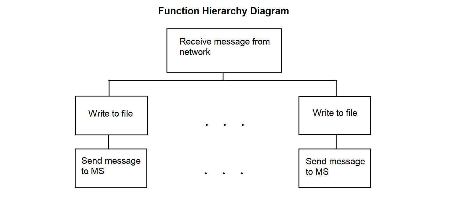
Figure 3.137

3.4.23. Driver for Receiving Data in SP from Central Link

The driver for receiving information in SP from the communication line with the center operates within the SP. It is intended to ensure the reception of information from the communication line with the center and its recording into PY for subsequent transmission via PC. The driver uses the bit-stuffing operation with zero deletion.

The necessity of bit-stuffing is as follows. In the absence of data to transmit over the network, the line-interface processor at the sending end outputs a continuous sequence of fill characters of the form 01111110. Data messages—which may themselves contain the fill character—are interleaved into this sequence. To distinguish an informational character from a fill character in the data stream, the sender inserts a zero after any sequence of five consecutive ones.

At the receiving end of the link, the incoming data stream is continuously monitored for five consecutive ones: if a “0” follows the five ones, it is discarded; if a sixth “1” follows, it indicates a received fill character.

The driver function hierarchy diagram is shown in Figure 3.138.

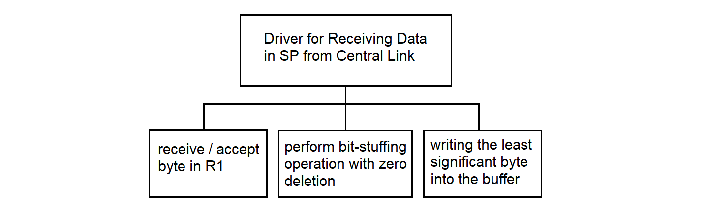
Figure 3.138

The pseudocode for the driver for receiving information in SP from the center’s communication line is shown in Figure 3.139.

; Driver for Receiving Information
; This algorithm processes the incoming data stream, performs bit-stuffing removal,
; and writes the result to a buffer
; CRC/flag frame checks are performed in PC software,
; this code handles only byte-wise reception and bit-stuffing removal.

; Block: Initialization of buffer and counters
output_buffer := empty         ; Buffer for storing processed bytes
C := array of zeros [0..15]    ; Array of counters:
                               ;   C[R4] — counter for processed bits in R4
                               ;   C[R3] — counter for consecutive 1s in R3
output_bit_buffer := 0         ; Bit buffer for accumulating processed bits
output_bit_count  := 0         ; Number of bits in output_bit_buffer
R1 := 0     ; Register for reading data byte, bit-stuffing operations
R2 := 0     ; Register for transferring byte to buffer, holds remainder from R1
R3 := 0     ; Number of bits set to 1 after 0 (from LSB to MSB)
R4 := 0     ; Register for remaining bits not yet transferred to buffer
R5 := 0     ; Value of previous remainder
R6 := 0     ; Auxiliary register
R7 := 0     ; Counter of processed bits

; Block: Main loop for processing the data stream
WHILE data available on communication line
; Block: Reading data from communication line
Read data byte from communication line
R1 := data byte                    ; Save the read byte in R1

; Block: Checking the byte type
IF data byte is informational THEN
; Initialization for processing an informational byte
R5 := 8                            ; Number of bits in a byte
R4 := 0                            ; Counter of processed bits

; Read the next byte and combine it with R1
Read data byte from communication line
R1 := (R1 << 8) OR data byte  ; Combine two bytes in R1 (16 bits)

; Block: Performing bit-stuffing removal
CALL "Bit-Stuffing Zero Deletion" with R1
; After the call, R1 contains the processed data,
; R4 — number of processed bits (must be set by subroutine, 0 to 15),
; result_pos — number of bits in the result
IF R4 > 15 THEN
R4 := R4 % 16                 ; Ensure R4 stays within bounds for C[R4]
END IF

; Block: Accumulating processed bits

IF result_pos > 16 THEN
 result_pos := 16  ; Prevent overflow
END IF
output_bit_buffer := (output_bit_buffer << result_pos) OR R1
output_bit_count  := output_bit_count + result_pos

; Block: Writing to buffer if 8 or more bits are accumulated
WHILE output_bit_count >= 8
byte_to_write := (output_bit_buffer >> (output_bit_count - 8)) AND 0xFF
Write byte_to_write into buffer
output_bit_count  := output_bit_count - 8
output_bit_buffer := output_bit_buffer AND ((1 << output_bit_count) - 1)
END WHILE

; Block: Additional bitwise filtering of R1
; This block may be masking six consecutive 1s (needs clarification);
; consider moving to a separate procedure if not required for bit-stuffing
R3 := 0                        ; Reset counter for 1s after 0
loop_counter := 1              ; Separate loop counter to avoid C[0] access
WHILE loop_counter <= 8
IF loop_counter < 5 THEN
bit := (R1 >> (R7 % 16)) AND 1 ; Check bit at position R7 (with limit)
IF bit = 1 THEN
R3 := R3 + 1                         ; Increment R3 if bit is 1
loop_counter := loop_counter + 1
ELSE
R3 := 0                                   ; Reset R3 on 0 bit
loop_counter := loop_counter + 1
END IF
ELSE
R6 := R1
R6 := R6 >> C[R4]
R6 := R6 >> max(0, C[R4] - 1)  ; Double shift, possibly 
;for masking 6 consecutive 1s
R1 := R1 AND R6
loop_counter := loop_counter + 1
END IF
IF R3 > 0 THEN ; Avoid accessing C[0]
C[R3] := C[R3] + 1 
END IF  
R7 := R7 + 1                 ; Increment processed bits
END WHILE
; Block: Bit distribution after bit-stuffing and processing
IF R4 < R5 THEN
R2 := R1
R5 := 8 - R4
ELSE
; Transfer the least significant R5 bits from R1 
; to the most significant bits of R2
IF R5 = 0 THEN
R2 := 0                         ; Avoid shift by 8 when R5 = 0
ELSE
R2 := (R1 AND ((1 << R5) - 1)) << (8 - R5)
END IF
R1 := R1 >> R5
Write the least significant byte of R2 into buffer
R2 := R1
R5 := max(0, min(8, 8 - R4 + R5))  ; R5 limited to [0, 8]
                                   ; to [0, 8] to prevant overflow
END IF

ELSE   ; Block: Processing control bytes
Write data byte into buffer
END IF
END WHILE

; Block: Writing remaining bits
IF output_bit_count > 0 THEN
byte_to_write := (output_bit_buffer << (8 - output_bit_count)) AND 0xFF
Write byte_to_write into buffer
END IF

The bit-stuffing operation with zero deletion in pseudocode is shown in Figure 3.140.

; Bit-Stuffing Zero Deletion Operation
; This algorithm performs bit-stuffing removal (deleting a zero after five ones)
; Input: R1 (16-bit register with data; larger inputs require 32-bit result)
; Output: R1 (processed data), R4 (number of processed bits,
; including skipped stuffing zeros, may exceed 16),
; result_pos (number of bits in the result)

; Block: Initialization of variables
ones_count := 0        ; Counter of consecutive ones
processed_bits := 0    ; Counter of processed bits
result := 0    ; Result after bit-stuffing removal (use 32-bit if result_pos > 16)
result_pos := 0        ; Position in the resulting bit stream
i := 0                 ; Bit position counter
skip_next := FALSE     ; Flag to skip the next bit (stuffing zero)

; Block: Processing all 16 bits in R1
WHILE i < 16
bit := (R1 >> i) AND 1
processed_bits := processed_bits + 1

    ; Determine whether to copy the current bit to the result
copy_bit := TRUE

IF bit = 1 THEN
ones_count := ones_count + 1
IF ones_count = 5 AND i < 15 THEN
next_bit := (R1 >> (i + 1)) AND 1
IF next_bit = 0 THEN
copy_bit := TRUE          ; Fifth "1" is already copied
skip_next := TRUE         ; Flag to skip the next bit
processed_bits := processed_bits + 1 ; Account for the skip
ones_count := 0
END IF
END IF
ELSE
ones_count := 0
END IF
ELSE
ones_count := 0
END IF

IF copy_bit THEN
IF bit = 1 THEN
result := result OR (1 << result_pos)
END IF
result_pos := result_pos + 1
END IF

IF skip_next THEN
i := i + 2                    ; Skip the stuffing zero (step +2)
skip_next := FALSE
ELSE
i := i + 1                    ; Normal step
END IF
END WHILE

; Block: Updating output values
R1 := result
R4 := processed_bits

; Block: Return control to the driver
RETURN R1, R4, result_pos
    

3.4.24. Driver for Receiving Data from PC to SP for Center Communication Lines

The driver for receiving information from PC to SP for the communication line with the center operates within the SP. The driver receives information addressed to the collection center from the communication line with the PC. The received information, after the bit-stuffing operation, is written to the mailbox buffer.

The driver hierarchy diagram is shown in Figure 3.141.

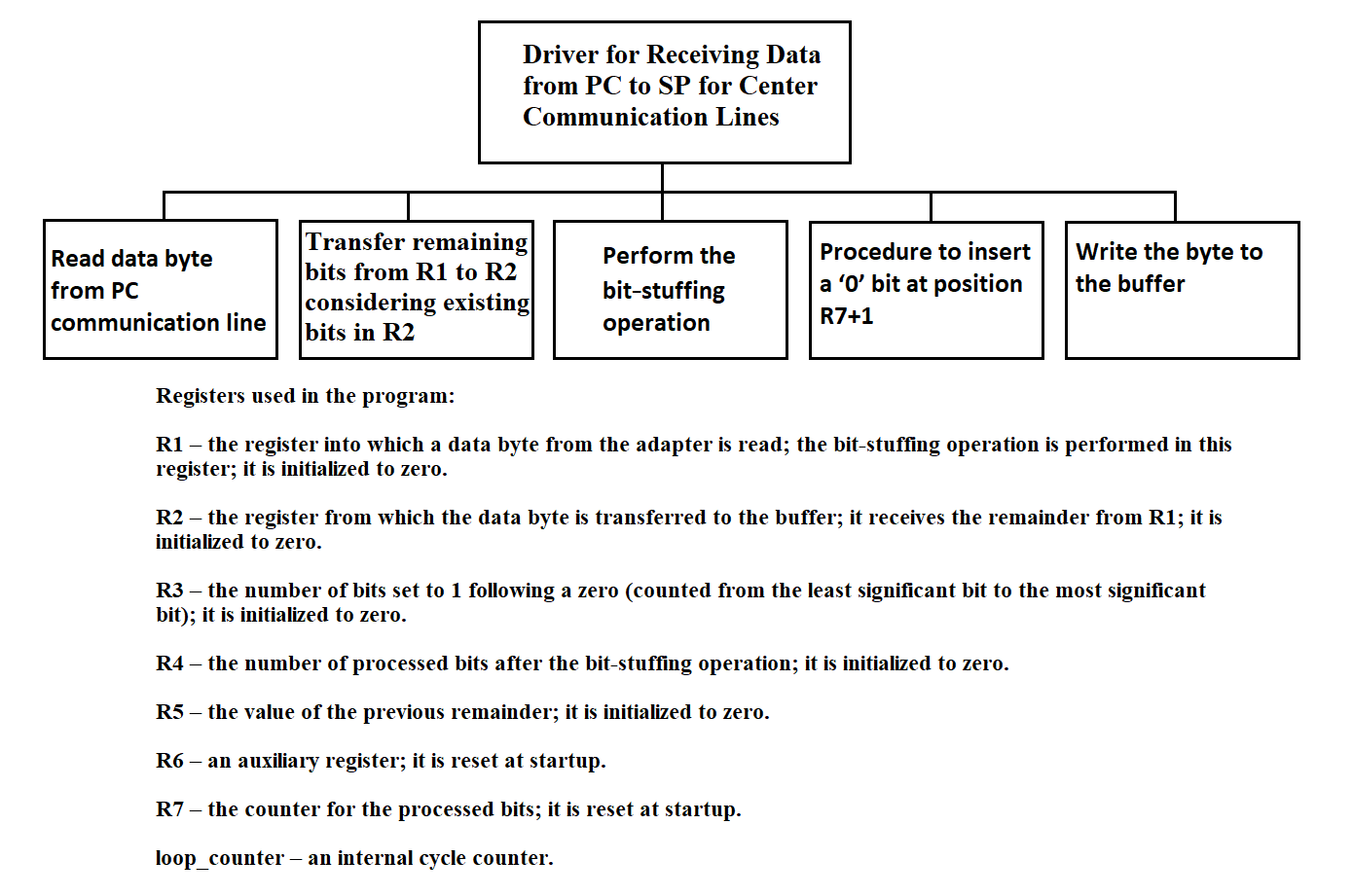
Figure 3.141

The driver for receiving information from PC to SP for the communication line with the center is shown in Figure 3.142.

DISABLE interrupts
READ a data byte from the chip into R1
MOVE R4 to R5
PERFORM the bit-stuffing operation in R1
R3 ← number of ones after the first zero
WRITE the number of “extra” bits into R4
R4 := R4 + R5
CALL “Transfer part of byte from R1 to R2 taking the remainder in R2 into account”
WRITE the lower byte of R2 to the buffer
SHIFT the upper byte of R1 right by 8 − R4 bits
IF R4 = 8 THEN
SHIFT R1 right by 8 − R4
WRITE the lower byte of R1 to the buffer
END IF
ENABLE interrupts
    

Procedure: transferring part of a byte from R1 to R2 taking into account the remainder in R2 is shown in Figure 3.143.

MOVE the lower byte of R1 into the upper byte of R2
SHIFT the upper byte of R2 left by C(R4) bits
OR the lower and upper bytes of R2
STORE the result in the lower byte of R2
    

Procedure: perform bit-stuffing operation

C(R7) := 1
C(R8) := 1
WHILE C(R8) ≤ 8 DO
IF C(R3) = 5 THEN
IF bit (R7 + 1) in R1 is 1 THEN
Insert a 0 at position R7 + 1
C(R7) := C(R7) + 1
R3 := 0
END-IF
END-IF
C(R7) := C(R7) + 1
Check bit N; if it is 1 then C(R3) := C(R3) + 1
C(R8) := C(R8) + 1
END-WHILE
    

Procedure for inserting the digit 0 at position R7 + 1

COPY R1 to R6
SHIFT R1 right by R7
SHIFT R1 left by R7 + 1
SHIFT R6 left by 16 − R7
SHIFT R6 right by 16 − R7
AND R1 with R6, store the result back to R1
    

R4 := R4 + R5

Shift upper byte of R1 right by (8 − R4)

R4 + R5 > 8

3.4.25. Program for Transmitting Data from the Center to the PC

The program for transmitting information from the center to the PC operates within the SP. When using a ring buffer to store information in the mailbox for all channels, regardless of the type and nature of the information, a unified read and write operation to the buffer is used.

Figure 3.146

The pseudocode for the program for transmitting information from the center to the PC is shown in Figure 3.147.

READ byte from buffer  
TRANSMIT data byte
    

3.4.26. Program for Transmitting Data from SP to the Center

The program for transmitting information from SP to the center operates within the SP. When using a ring buffer to store information in the mailbox for all channels, regardless of the type and nature of the information, a unified read and write operation to the buffer is used. The hierarchy diagram of the program function is shown in Figure 3.148.

Figure 3.148

The pseudocode for the program for transmitting information from SP to the center is shown in Figure 3.149.

READ byte from buffer  
TRANSMIT data byte
    

3.4.27. Driver for Receiving Data into SP from Center Line in Byte-Stuffing Mode

This section discusses a variant for ensuring the transparency of transmitted data using byte-stuffing. It is assumed that in the absence of data, a padding sequence of the form DLE STX is continuously transmitted to the network. At the receiving end, this sequence is programmatically discarded. If a symbol matching DLE appears randomly in the data stream, it is duplicated at the transmitting end and removed at the receiving end.

The driver operates in the SP OS. It is designed to receive information transmitted from the collection center and write it to the SP mailbox for subsequent transmission to the PC. In the byte-stuffing variant, information from the communication line with the center arrives byte by byte; during pauses, padding bytes in the form of DLE STX arrive. Two DLE symbols may occur in the information text, one of which must be discarded.

The hierarchy diagram of the driver for receiving information in SP from the communication line with the center is shown in Figure 3.150.

Figure 3.150

The driver for receiving information in SP from the communication line with the center in the byte-stuffing variant is shown in Figure 3.151a.

; ----------------  Data Processing from Communication Line  ----------------
; This algorithm reads data from the communication line, handles DLE flags,
; and writes to the buffer.
; Note: it removes stuffing based on the DLE-flag logic.

READ_DATA_BYTE                         ; Read a data byte from the line
COUNTER ← COUNTER + 1                  ; Increment byte counter
CALL VOSST_PROCEDURE                   ; Call VOSST as requested

IF FLAG_DLE = 1 THEN
IF DATA_BYTE = DLE THEN
WRITE_BUFFER DATA_BYTE          ; Pass stuffed DLE to buffer
FLAG_DLE ← 0                         ; Clear flag
END IF
FLAG_DLE ← 0                ; Discard stuffing symbol (e.g. ‘STX DLE STX’)
ELSE
IF DATA_BYTE = DLE THEN
FLAG_DLE ← 1                         ; Next byte is stuffed
ELSE
WRITE_BUFFER DATA_BYTE          ; Regular data byte
FLAG_DLE ← 0                         ; Extra robustness
END IF
END IF

The recovery procedure is shown in Figure 3.151b.

;  ---------------- Procedure: VOSST Procedure ----------------
; This procedure handles register preservation, mailbox buffer management,
; and counter reset

SAVE_REGS                                  ; Save registers

DS ← ADDRESS_OF_MAILBOX_0                  ; Set DS pointer to the beginning
                                           ; of all ring buffers in mailbox

IF FLAG_DLE = 1 THEN                     ; Check DLE flag
IF DATA_BYTE = SYN THEN           ; Check SYN control byte
COUNTER ← 0                        ; Reset counter at start of packet
END IF
END IF

IF COUNTER overflowed THEN                ; Timeout / overflow detection
COUNTER ← 0                        ; Prevent overflow
CHIP_ADDR ← FIND_TARGET_CHIP()     ; Locate required chip
OUTPUT 0DB7h TO CHIP_ADDR          ; Send sync / reset command
END IF

RESTORE_REGS                                ; Restore registers
RET                                         ; Return from procedure

3.4.28. Driver for Receiving Data from PC into SP for Transmission over Center Line in Byte-Stuffing Mode

The driver operates in SP. It receives data bytes from the PC and transfers them to the mailbox buffer for subsequent transmission to the communication line with the center. Upon receiving the DLE symbol, it is duplicated. The hierarchy diagram is shown in Figure 3.152.

Figure 3.152

The driver for receiving information from the PC to the SP for the communication line with the center in the byte-stuffing variant is shown in Figure 3.153.

READ data byte from microcircuit
IF data byte is DLE
WRITE DLE to buffer
END IF
WRITE byte to buffer
    

3.4.29. Remote Concentrator Network Software Algorithm

The "COLLECTION" system provides the following functions using network software:

• transmission of measurement information from remote concentrators to the collection center for subsequent processing;
• exchange of organizational information.

The transmission of measurement information occurs in three modes:

• real-time forwarding;
• forwarding of delayed information;
• playback mode.

The exchange of organizational information includes:

• exchange of formalized messages;
• teleconferences;
• forwarding of structured documents;
• forwarding of binary files.

The subroutines of the network software must ensure the handling of connection breaks and subsequent restorations of the access path through the network environment, performing all necessary actions to restore inter-task interaction.

3.4.29.1. Real-Time Measurement Data Transfer

The main characteristic of the real-time mode is the transmission of information at the rate of its arrival.

Information for the transport subsystem comes from the software directly interacting with measuring instruments through the Synchronization Processor of RC. The consumers of information are several processes in the node of the collection center. One of them (mandatory) is the registrar process, which writes all received information to disk drives. The remaining processes can be loaded in various operating modes as needed.

The following programs support the output of messages to the communication line in real time:

• message queue formation;
• transmission of messages from the queue to the network.

For the functional description and algorithms of these programs, see sections 3.4.29.5 and 3.4.29.6 respectively.

3.4.29.2. Transfer of Delayed Real-Time Data

Since the transmission of measurement information occurs under conditions of potentially unreliable real-time channels, communication interruptions with individual nodes are possible. These interruptions can occur intentionally, at the initiative of a human operator controlling the information exchange process, or due to technical reasons that occurred in the communication channel. In any case, these situations must be tracked and handled by network environment subroutines.

Measurement information transmitted to the collection center in real time is simultaneously recorded on an external RC storage medium. If it is impossible to establish communication with the center, the information that is delayed by the real-time moment is written to the RC disk and supplemented with a flag characterizing it as delayed, and then transmitted to the collection center in relative time mode.

The transportation of delayed information (DI) takes place in 2 stages:

• formation of files containing delayed information;
• transfer of these files to a remote node and their registration on the disk of the collection center's file server.

The first stage is implemented by a software module for generating files containing delayed information, written in C (see section 3.4.29.7). In the second stage, a Shell language command file is executed, which includes a call to the standard network user file transfer utility FTP (see section 3.4.29.8).

3.4.29.3. Playback Mode Data Transmission

In playback mode, information is transmitted in relative time. The transmission speed is determined only by the bandwidth of the communication line. When operating in playback mode, the information is already in the external memory of the RC, which is achieved by a combination of the real-time mode for the RC and the absence of communication with the center.

A Shell language command file is used to implement the transmission of information in playback mode (see section 3.4.29.9).

3.4.29.4. Organizational Data Transmission

This function is activated by a program from the collection center. Currently, it has only been outlined and is intended to support the following operations:

• exchange of one-time formalized messages;
• inter-terminal exchange (teleconferencing) between network subscribers;
• forwarding of structured documents;
• forwarding of pre-calculated data.

All these functions can be performed using the "e-mail" service available to every operator using the "COLLECTION" system terminal.

The exchange of organizational data can be carried out either immediately (for example, during inter-terminal interactions) or in a delayed mode (for example, during file exchange).

When exchanging one-time formalized messages, the network environment provides the following services:

• the ability to prepare and modify a message file;
• viewing formalized messages and selecting the messages necessary for forwarding;
• inter-terminal exchange of pre-prepared messages;
• password-based access for users to the "e-mail" service, including the registration procedure;
• maintenance and, if necessary, display of a list of active users and their pseudonyms;
• confirmation of successful message delivery.

Inter-terminal information exchange is organized in keyboard input mode, but the inclusion of pre-prepared text files is allowed.

The structured document forwarding system involves the transfer of files from one user to another, regardless of the latter's activity. The transferred files are entered into a special catalog and can then be selected by the recipient if necessary. Upon registration, the user receives a notification about the availability of files addressed to them. The user can view annotations for incoming files and select the necessary documents in their catalog.

Document transfer is carried out using a queue. All files requiring forwarding are placed in the queue, and the "e-mail" monitor, viewing the request file, tries to establish a logical channel at the recipient's node and send the corresponding file to it. After successful transfer, the request record is deleted from the queue, and the original file is removed.

Pre-calculated data can be binary, text, or other files of arbitrary internal structure. Forwarding occurs "blindly" in binary form without any changes. The sender may have the option to accompany the information with a corresponding password. Thus, when implementing the function of organizational data exchange, the network environment must ensure the following:

• organize the operation of the "e-mail" system;
• preparation of source data for the transmission of fixed messages from one remote node to another;
• inter-task communication in the remote nodes of the network.
• support for the execution of subroutines for receiving, displaying, and confirming messages by a remote user;
• organization of access to the "e-mail" service through a password system;
• the presence of an additional subroutine that provides the user with information about mail subscribers and the specific terminal numbers they are working with.

3.4.29.5. Message Queue Formation Program Algorithm

The message queue formation program performs the following functions:

• creates a message queue;
• places a message in the queue.

Input information: the address and length of the message, which come from the message processing programs from MS "Vega" (see section 3.3.1) and "Kama" (see section 3.3.2).

The hierarchy diagram of the message queue formation program function is shown in Figure 3.154.

Figure 3.154

The message queue formation program works with the message queue identifier msgid.

The identifier msgid corresponds to the message queue and the data structure msgid_ds.

The data structure msgid_ds of the message queue contains:

• the msg_perm structure of rights for operations on the message queue,
• msg_first - a pointer to the first message in the queue,
• msg_last - a pointer to the last message in the queue,
• msg_cbytes - the current number of bytes in the queue.
• msg_qnum - the number of messages currently in the queue,
• msg_qbytes - the maximum number of bytes allowed in the queue,
• msg_lspid - the process identifier that last performed the msgsnd operation,
• msg_lrpid - the process identifier that last performed the msgrcv operation,
• msg_stime - the time of the last msgsnd operation,
• msg_rtime - the time of the last msgrcv operation,
• msg_ctime - the time of the last modification operation,
• msg_qnum - is the number of messages currently in the queue,
• msg_qbytes - is the maximum number of bytes allowed in the queue,
• msg_lspid - is the identifier of the process that last performed the msgsnd operation,
• msg_lrpid - is the identifier of the process that last performed the msgrcv operation,
• msg_stime - is the time of the last msgsnd operation,
• msg_rtime - is the time of the last msgrcv operation,
• msg_ctime - is the time of the last change operation.

The msg_perm structure, which specifies the permission for operations on messages, includes the following members:

• identifier of the user who created the queue;
• identifier of the group of users who created the queue;
• user identifier;
• group identifier.

The permission type for operations on messages is interpreted as follows:

• 00400 - read by owner
• 00200 - write by owner
• 00060 - read, write by group
• 00006 - read, write by others

The algorithm of the message queue formation program is presented in Figure 3.155.

SET first entry flag of the program  
PRENTRY := 0  
SET program busy flag  
PRG := 1  
IF queue IS NOT created THEN
CREATE and GET its identifier msgid
SET flag PRENTRY := 1
SET message counter qnum := 0
ELSE
IF queue IS ALREADY full THEN
SET overflow flag PR := 1
ELSE
PUT message into queue
qnum := qnum + 1
SET flag PRG := 0
END IF
END IF
    

The message queue formation program uses the following system calls:

• msgget get the message queue identifier msgid;
• msgsnd send a message to the queue;
• msgrcv read a message from the queue.

3.4.29.6. Network Message Transmission Program Algorithm

The program for transmitting messages from the queue to the network transmits a message from MS "Vega" or "Kama".

The program for transmitting messages from the queue to the network does not analyze the content of the messages. The program functions are shown in Figure 3.156.

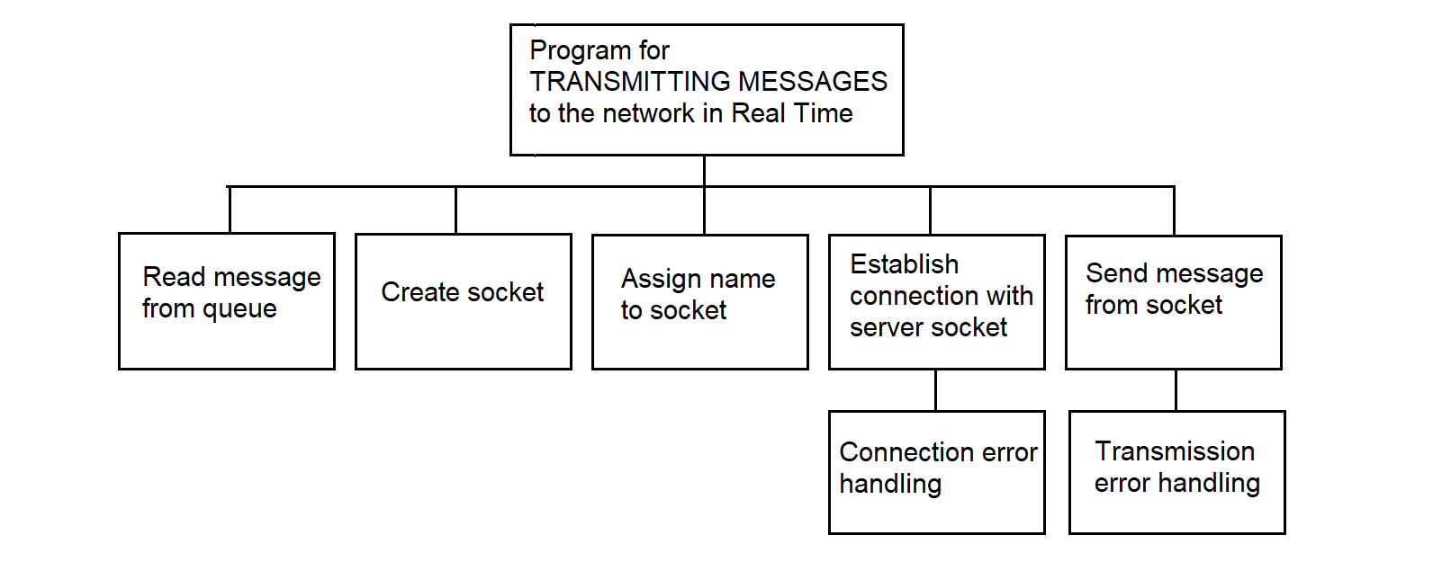
Figure 3.156

The program for transmitting messages from the queue to the network is executed in the TCP/IP of Interactive Unix environment using sockets. A socket is a final addressable communication point (block) within a program, associated with one of the exchange processes. A named pair of sockets uniquely defines the connection between the switched nodes (collection center and RC). The interaction of processes in the exchange takes the form of a client-server connection; the program for transmitting messages from the queue to the network is the client, and the reception program at the collection center is the server, with the client being an active process and the server being a passive process.

The client uses the following network calls:

• socket
• bind
• connect
• write
• read
• close

The client and server use the same network calls for receiving and sending messages and different network calls when establishing a connection. On the server, after creating its socket, two network calls must be issued to establish a connection with the client:

• listen, indicates readiness to listen for incoming connection requests;
• accept, is used to accept a connection (connect call) from the client.

The call returns a connection acknowledgment to the client. Once the connection is established, data can be transmitted/received using the following calls: write, read, send, recv.

The send, recv calls are identical to write, read, except for the flags argument. If there are no messages on the server socket, the recv call waits until these messages arrive.

The output program initiates the exchange, i.e., acts as an active client. The client establishes a connection with the collection center's program server using the connect network call, whose parameters are: socket and the destination address.

The algorithm for sending a message via a socket is shown in Figure 3.157.

CREATE SOCKET  
ASSIGN NAME TO SOCKET  
ESTABLISH CONNECTION  
ACCEPT CONNECTION ON SOCKET  
WHILE THERE ARE MESSAGES IN THE QUEUE  
SEND MESSAGE
IF confirmation IS NOT received THEN
SET delayed information flag
END IF
END WHILE
    

3.4.29.7. Program for Generating Delayed Information Files

This program implements the following functions:

• selection of files registered during specific tests. The selection of files is based on the date specified by the human operator, from which it is necessary to perform the post-session transfer of delayed information.
• viewing the contents of the file and selection based on a specific attribute of records containing delayed information;
• formation of new files containing delayed information in the COLLECTION/DATA/SERVER/TMP directory.

Input parameters: Flag - indication of the presence of DI;

Output information: files containing DI are placed in the COLLECTION/DATA/SERVER/TMP directory.

When the program is activated, a request appears on the screen,

on which the human operator must enter the date, starting from which files will be selected to identify DI in them.

The date is entered in DD/MM/YY format.

The last line of the screen contains a hint indicating the meaning and format of the entered date.

The hierarchy diagram of the function of the software module for forming delayed information files is shown in Figure 3.158.

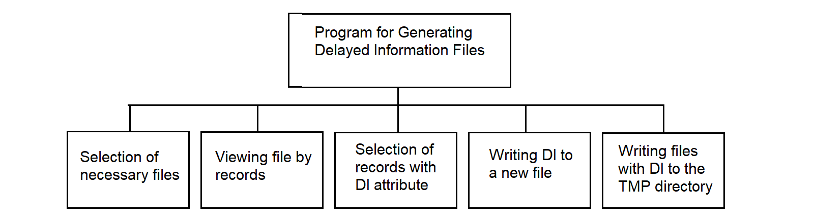
Figure 3.158

The description of the program for forming files with delayed information in pseudocode is presented in Figure 3.159.

; Algorithm “Extract DI Records” — copy DI-marked records to separate file

IF DI = yes THEN
IF directory COLLECTION/DATA/SERVER/TMP DOES NOT exist THEN
CREATE directory COLLECTION/DATA/SERVER/TMP
END IF

WHILE there are files in COLLECTION/DATA/SERVER directory
OPEN file from COLLECTION/DATA/SERVER directory
OPEN file for writing DI

WHILE NOT end of file
READ record into buffer
IF 1st character of record = DI indicator THEN
WRITE record to DI file
INCREMENT record pointer in DI file by 1
END IF
INCREMENT record pointer in source file by 1
END WHILE

CLOSE file from COLLECTION/DATA/SERVER directory
CLOSE file for writing DI
WRITE file to COLLECTION/DATA/SERVER/TMP directory
GET next file from COLLECTION/DATA/SERVER directory
END WHILE
END IF

The generation of file names containing DI occurs as follows: the symbol "O" is added as the first symbol to the name of the original file containing the measurement information.

3.4.29.8. Command File Algorithm for Transmitting Delayed Information

The Shell language command file works as follows:

1. Establishes a connection with the remote node using the OPEN command of the FTP utility.
2. Sets the COLLECTION/DATA/SERVER/TMP directory as the current one.
3. Writes a list of all files in the COLLECTION/DATA/SERVER/TMP directory to the DirTmp variable.
4. Organizes a loop while the value of the DirTmp list variable is not empty.
5. The following operations are performed in the loop body:
   • the value of the DirTmp list element is passed as a parameter to FTP;
   • the PUT command of the FTP file transfer utility is executed;
   • after a message about the normal completion of the file transfer is issued, this file is deleted from the directory;
   • the pointer is incremented, and a jump to the beginning of the loop is performed.
6. Closes the connection with the remote node using the CLOSE command of the FTP utility.

Subsequently, the transferred files can be joined to files containing measurement information of this type, or they can be processed independently.

3.4.29.9. Command File Algorithm for Information Transmission in Playback Mode

The algorithm of the command file for transmitting information in playback mode is as follows:

1. The content of the file containing the list of files for transmission in playback mode is assigned to the list variable Flist.
2. A connection is established with the remote node using the OPEN command of the FTP utility.
3. A loop is organized while the list variable Flist is not empty.
4. In the loop body:
   • the file name, which is selected from the list variable Flist, is passed as a parameter to the FTP file transfer utility.
   • the file is transferred to the remote node using the PUT command of the FTP utility and written to the disk of the collection center's file server.
5. The connection with the remote node is closed using the CLOSE command of the FTP utility.

4. TECHNICAL AND ECONOMIC JUSTIFICATION

A feature of the software being developed for the RC is the widespread use of standard software and applied technical means. The operating environment and network tools supplied for IBM PC-type personal computers are used.

This approach is justified from the point of view of development costs, since in modern information systems, software development costs account for up to 80% of the total cost of work.

The method of structured programming is used in software development. This method reduces labor costs in software development and its operation. In addition, important quality criteria for the software become its clarity, reliability, and ease of maintenance, as well as the ability to accurately plan work.

LIST OF ABBREVIATIONS

• BCC - Block Check Character
• CB - Check Buffer
• CC - Collection Center
• CL - Communication Line
• CPU - Central Processing Unit
• CS - Control Symbols (service symbols)
• CSR - Command/Status Register
• CSEQ - Control Sequence
• DLE - “Data Link Escape” control symbol
• ENQ - “Enquiry” control symbol (“Who’s there?”)
• EOT - “End of Transmission” control symbol
• ETB - “End of Transmission Block” control symbol
• ETF - End-of-Transmission Flag
• ETX - “End of Text” control symbol
• FEF - Format Error Flag
• II - Information Index
• LD - Late Data
• LFSR - Linear Feedback Shift Register
• MB - Mailbox
• MM - Main Memory
• MP - Measuring Point
• MS - Measuring System
• PC - Personal Computer
• PIC1 - Programmable Interrupt Controller 1
• PIC2 - Programmable Interrupt Controller 2
• RAM - Random-Access Memory
• RC - Remote Concentrator
• ROM - Read-Only Memory
• RSI - Radial Serial Interface
• SOR - Statement of Requirements (tactical & technical)
• SP - Synchronization Processor
• SSR - Specific (private) Technical Assignment
• STC - Scientific and Technical Center
• STS - Special Technical Specification (see also SSR)
• STX - “Start of Text” control symbol
• SW - Software
• SYN - Synchronization control symbol
• TS - Technical Specification (see also SOR)
• US - “Unit Separator” control symbol

LIST OF USED DOCUMENTS

1. Unified system of program documentation. Moscow: publishing house of standards 1985
2. GOST 17422-72
3. GOST 19767-74
4. J. Hughes, J. Michtom Structural approach to programming Moscow: Mir 1980

APPENDIX A. METHOD FOR CONSTRUCTING THE OPTIMAL TOPOLOGY OF THE PHYSICAL STRUCTURE OF A MESSAGE EXCHANGE COMPUTING NETWORK

A.1. Traditional Topologies of the Message Exchange Computing Network

The topology of a message exchange computing network is its physical structure—that is, the way in which Measuring Systems (MS) are connected to data collection nodes. The term “topology” is borrowed from geometry and is used to describe the connectivity pattern of such a distributed network. The traditional topologies, as shown in Figure A.1, include:

1. hierarchical (tree),
2. horizontal (bus),
3. star,
4. ring,
5. mesh.

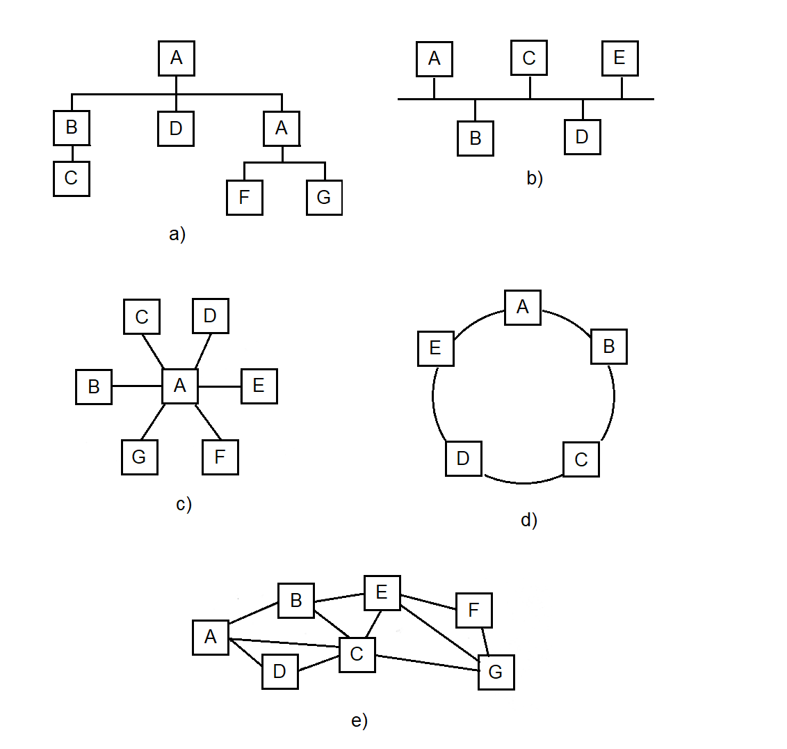
Figure A.1 Traditional network topologies.

Each of these configurations has been applied in various technical systems, ranging from military complexes to civilian surveillance and telemetry systems.

A.1.1 Structure of the Message Exchange Computing Network

In the context of topology construction, we consider systems where multiple distributed Measurement Systems (MS) transmit data to the central node — the Collection Center Concentrator (CCC), either directly or via intermediate nodes — Remote Concentrators (RC).

This architecture is typical for systems operating across large geographic areas: from missile and space complexes, where MS are placed along the flight trajectory, to meteorological services, where MS placement is determined by regional geography.

In all cases, the network has a hierarchical structure:

• upper level — Collection Center Concentrator (CCC),
• middle level — Remote Concentrators (RC),
• lower level — Measurement Systems (MS).

A.1.2 Topology of the Message Exchange Computing Network

A Message Exchange Computing Network is built as a hierarchical structure in which each lower-level element transmits information through one or more intermediate nodes to the central collection node — the Collection Center Concentrator (CCC).

Measurement Systems (MS) are connected either directly to the CCC or via one of the Remote Concentrators (RC), which are installed at selected points in the network. This configuration allows for significant reduction in the total cost of communication lines and simplifies interfacing between heterogeneous components. In this way, the Remote Concentrator (RC) serves as a universal element of the network’s physical structure, ensuring the integration of any MS into a unified hierarchy.

The key principle is message-based communication logic: each node in the network transmits not raw data streams but meaningful messages that may contain telemetry, control commands, or measurement frames. The architecture itself is independent of specific hardware or communication protocols.

A critical feature: all messages are processed with priority, which ensures timely handling of mission-critical data and robustness of the system under high load conditions.

A.2. Method for Constructing the Optimal Topology of the Physical Structure of a Message Exchange Computing Network

“Technical problems generally present themselves as optimization problems, for two main reasons. First, the limitation of resources and the diversity of our needs compel us to use resources carefully and to weigh our needs. Second, the production and use of technical means lead not only to desirable but also to undesirable consequences, so good solutions to technical problems are always expected to optimize actual benefits.” [3]

Let us consider the well-known methods for designing data transmission network topologies. According to [1], the methods are classified into:

1. designing the topology of a communication subnetwork to support traffic generated by terminals, including the selection of node locations, communication lines, and bandwidth capacity for each line;
2. designing a local access network, i.e., a set of communication lines connecting terminals to the entry nodes of the subnetwork.

Taking into account the territorial and geographical distribution of measurement sites and Measurement Systems (MS), e.g., along the test flight path of an ICBM, it is natural to consider the network as a local access network.

There are two possible ways to connect MS: either directly to the Collection Center Concentrator (CCC) or via a Remote Concentrator (RC). If such a choice is available, it opens up the opportunity to minimize the cost of the information processing system for collecting incoming telemetry data.

At the same time, using previously introduced simplifications and assumptions, Nikolaiev extended the well-known "addition" method, proposed by J. Martin and described by M. Schwartz [4], to new classes of objects and systems — specifically, the Message Exchange Computing Network and RCs. The optimal-cost topology of the "Collection" telemetry data collection system for the Plesetsk Cosmodrome was also developed by the author using this "addition" method, as confirmed by implementation reports.

A comprehensive and precise solution to the topology synthesis problem is a complex task. A preferred approach is to develop and utilize ready-made algorithms and combine them into a software package for topological synthesis. An example of such a package is the "Software and Methodological Toolkit for Automated Design of Microelectronic Equipment Topology," developed by Nikolaiev in collaboration with Voloshyn [2].

A more formal formulation of the problem is as follows: a set of \( N \) MS must be connected via RCs to the CCC. Given a set of MS and a set of possible RC placement locations, it is necessary to select an appropriate subset and determine which MS are connected to which RCs, and which are connected directly to the CCC. The RC may be co-located with the MS itself, as in the "Vega" systems.

The cost of installing an RC includes equipment cost, commissioning cost, and the cost of the communication line between the RC and the CCC. It is assumed that no more than \( N_{\text{max}} \) MS can be connected to a single RC. For example, the NI525 kit includes 6 MS, while the “Briz” meteorological concentrator used in the State Hydrometeorological Service of Ukraine supports 45 MS.

The CCC is assumed to have unlimited capacity. Let the cost of connecting the \( i \)-th MS to the \( j \)-th RC be denoted as \( C_{ij} \), where \( i = 1 \ldots N \), \( j = 0 \ldots N_K \) (with 0 corresponding to the CCC).

Let us define the exact expression for the total cost function \( S \) to be minimized. We introduce a variable...

Let us introduce the variable \( x_{ij} \), where

The variable \( y_j \) equals 1 if \( RC_j \) is installed and used, and \( y_j = 0 \) if \( RC_j \) is not installed. Alternatively, \( y_j = 1 \) if \( \sum_{i=1}^{N} x_{ij} > 0 \), and \( y_j = 0 \) otherwise. Thus, \( y_j = 1 \) if at least one MS is connected to the j-th RC.

Then the expression for the total cost to be minimized is as follows:

The first term defines the cost of the installed RCs, and the second term — the cost of the communication lines connecting MS to RCs. Minimization of the function \( S_{\Sigma} \) must be performed subject to constraints.

1)  \[ \sum_{j=0}^{N_K} x_{ij} = 1,\quad i = 1, N, \] which means that each MS must be mandatorily connected either to a remote concentrator (RC) or directly to the central concentrator (CCC).

2)  \[ \sum_{j=0}^{N_K} x_{ij} \leq N,\quad j = 1, \overline{N_K}, \] which means that no more than N MS can be connected to any RC.

The task is to determine the set of variables \( y_j \) and \( x_{ij} \) that minimize \( S_{\Sigma} \), subject to constraints 1) and 2).

If the integer constraint \( x_{ij} = 0 \) or \( 1 \) is replaced with a non-integer constraint

then the problem turns into a transportation problem of linear programming and can be solved, for example, by the simplex method.

It is known from the literature [14] that the solution obtained by the simplex method will be integer, i.e., \( x_{ij} \) will be equal to 0 or 1. Therefore, solving the problem without considering integer constraints will automatically lead to an optimal integer solution.

The complexity of solving the problem is determined by the dimensionality of the network. Therefore, for large networks, it is recommended to use heuristic algorithms such as “addition” and “removal” [83].

To clarify the use of heuristic methods for building the topology, let us consider an example of constructing a message exchange computing network using the “addition” method. There are eight measurement systems (MS) whose information must be collected at the central collection concentrator (CCC).

In this case, it is possible to install three remote concentrators (RC): \( K_1, K_2, K_3 \), which can gather information and forward it to the collection center.

Let us assume that the cost of installing an RC, including the cost of the communication line to the CCC, is (in conventional units):

The cost of communication lines between MS and nodes (CCC and RC) is defined by the elements of the matrix \( C_{ij} \).

The cost matrix of connections between measurement systems (MS) and nodes (CCC and RC):

The rows correspond to measurement systems (MS), and the columns represent nodes: column 0 corresponds to the central concentrator CCC, while columns 1, 2, and 3 represent the remote concentrators RC₁, RC₂, and RC₃, respectively.

Figure A.2 shows the set of stand-alone MS and RC, whose locations are known and used as initial data for constructing the topology of the message exchange computing network.

Initially, all measurement systems (MS) are connected to the central data collection concentrator (CCC):

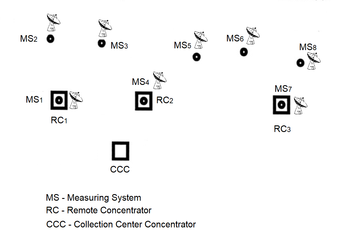
Figure A.2 The set of MS and RC as physical elements of the constructed
Message Exchange Computing Network.

Initially, only the proposed locations for installing the concentrators (RC) are known. The installation of RCs is carried out using an iterative scheme aimed at gradually reducing the total cost of the message exchange computing network.

This algorithm belongs to the class of steepest descent algorithms.

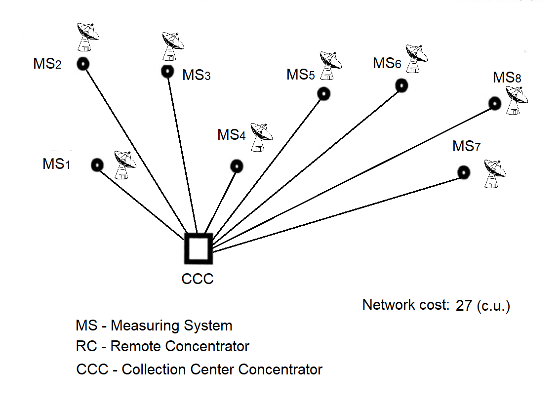
Figure A.3 Initial stage — connection of all MS directly to the CCC.

At the beginning of the problem solution, it is assumed that only the central data collection concentrator (CCC) is functioning, and all measuring systems (MS) are directly connected to it, as shown in Figure A.3.

The initial total cost of the star topology message exchange computing network is calculated by summing the elements of the zero column of matrix C:

$$ S_{\Sigma} = \sum_{i=1}^{8} C_{i0} = 27\ \text{c.u. (conventional units)} \tag{A.4} $$

Step 1. Install RCs sequentially at the measuring points and identify cost savings based on negative values of the differences:

$$ C_{ij} - C_{i0},\quad j = 1,3,\quad i = 1,8. \tag{A.5} $$

The difference values are shown in Table A.1. If RC₁ is installed with the connected measuring systems MS₁, MS₂, and MS₃, the total network cost would decrease to 25 units:

If the concentrator \( RC_1 \) is installed with the connected measuring systems \( MS_1 \), \( MS_2 \), and \( MS_3 \), the total network cost would decrease to 25 units:

\[ S_1 = \sum_{i \in \{3,4,5,7,8\}} C_{i0} + \sum_{i \in \{1,2,6\}} C_{i1} + f_1 = 25\ \text{c.u.} \tag{A.6} \]

If, instead of the first concentrator \( RC_1 \), the second concentrator \( RC_2 \) is installed, the total network cost will decrease to 18.5 units:

\[ S_2 = \sum\limits_{i \in \{2,3,7\}} C_{i0} + \sum\limits_{i \in \{1,4,5,6,8\}} C_{i2} + f_2 = 18.5\ \text{c.u.} \tag{A.7} \]

The network cost at the first step (with only one remote concentrator installed) will become minimal and equal to 17 units if, instead of the second concentrator \( RC_2 \), the third concentrator \( RC_3 \) is installed.

\[ S_3 = \sum_{i \in \{1,2,3,4\}} C_{i0} + \sum_{i \in \{5,6,7,8\}} C_{i3} + f_3 = 17\ \text{c.u.} \tag{A.8} \]

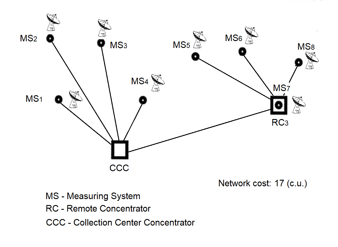
Figure A.4 First step of the "addition" algorithm: installation of RC.

Based on the calculated total cost of the message exchange computing network with one remote concentrator installed, it is concluded that the installation of the third concentrator \( RC_3 \) is the most cost-effective option, as it reduces the network cost by 10 units \( (27 - 17) \). The configurations yielding 25 and 18.5 units are not illustrated, as they are intermediate and less advantageous compared to the 17-unit configuration selected for further optimization.

Step 2. After installing RC₃, the next concentrator is added, and the feasibility of connecting either RC₁ or RC₂ is evaluated in terms of potential savings. All measuring systems (MS), including those already connected to RC₃, are considered. For this purpose, Table A.2 is compiled. Based on the negative values in Table A.2, it becomes clear that connecting measuring systems MS₁ and MS₂ to RC₁ results in a cost advantage. The cost savings are then verified:

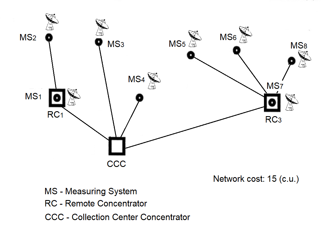
Figure A.5 Network topology after installation of the next RC.

Now we add the concentrator RC₂ and check whether its installation is justified. The differences are shown in Table A.3. Installing RC₂ results in cost savings by connecting to it the measuring systems denoted as P₄ and P₅. Let us verify the total cost of the network. It will amount to:

Figure A.6 Minimum cost network topology.

A.3. Message Exchange Network Topology: Step-by-Step Formation

← →

A.4. Conclusions

1. A message exchange computing network covering remote measuring systems (MS) is organized as a hierarchical structure, where the Collection Center Concentrator (CCC) is located at the top level, Remote Concentrators (RC) operate at the intermediate level, and MS are located at the bottom level. This organization is suitable for telemetry, meteorological, and other distributed systems operating in real time.
2. The methodology for constructing the optimal topology consists in adapting the "addition" method to a new class of tasks, where Remote Concentrators (RC) serve as universal nodes for integrating various measuring systems into a unified network based on priority message exchange.
3. The information concentrator technology has demonstrated the ability to transfer solutions from the military domain to civilian systems (meteorology, transportation, energy), highlighting its versatility and scalability.
4. For projects implemented using SCRUM or other agile methodologies, the calculator provides labor intensity estimates that align with the Waterfall method within an engineering accuracy of approximately ±5%. This makes the tool applicable even in modern agile development environments.
5. The labor intensity calculator on the main page condenses 39 years of engineering experience into algorithms. It reflects how my team of seasoned developers would implement your project, balancing labor intensity, team size, and deadlines. These numbers are not just estimates—they are backed by real-world systems that operate in extreme conditions: real-time military platforms where failure is not an option, and meteorological complexes that have been collecting data continuously for over 25 years, unaffected even by hurricanes. If you can do better—my experience has served as your springboard, and that is the highest success. … and that is the highest success. 👉 Try the calculator .

Genealogy of Information Concentrators

1991 — "Collection"
The concentrator passed qualification testing.

1993 — "Collection"
A cryptographically protected network was established between Plesetsk (Mirny) and Vorkuta.

1995 — "Collection"
The "Collection" system was put into operation: Severodvinsk — Mirny — Vorkuta.

1995 — "Unified Control Center"
Priority processing was introduced: control commands were handled with higher priority.

1997 — "Unified Control Center"
Adaptive control of antenna fields of geographically distributed radio engineering systems in real machine time during ballistic missile tests.

1998 — Connection of the modernized MS "Vega", Norilsk via a satellite channel and the "Crystal" equipment.

1999 — Meteorological Concentrator "Briz"

• On-the-fly message recoding and reformatting
• Extended priority scale
• Dynamic traffic control and direction switching
• Still in operation

2002 — SKNOU

• Advanced real-time mathematical computation capabilities
• Reduced traffic management functions due to the absence of specific requirements
• Real-time visualization of transmission status, computations, and satellite constellations

2014 — Urban Passenger Flow Accounting

• The concentrator is used as a key element of the real-time system in urban public transportation
• As a message switching node, the concentrator fully decouples physical devices from system logic, allowing flexible system architecture without limitations

References for Appendix A: Topology of the Message Exchange Computing Network

1. Мартин Дж. Планирование информационно-вычислительных систем. – М.: Радио и связь, 1982.
   Martin J. Planning of Information and Computing Systems. – Moscow: Radio i Svyaz, 1982.
2. Волошин А.Н., Николаев А.Н. Программно-методический комплекс проектирования топологии. – Киев: ИПРИ, 1991.
   Voloshin A.N., Nikolaev A.N. Software and Methodological Package for Topology Design. – Kyiv: IPRI, 1991.
3. Шеффлер И. Условия механизации мышления. – М.: Прогресс, 1978.
   Scheffler I. Conditions for Mechanization of Thinking. – Moscow: Progress, 1978.
4. Шварц М. Компьютерные системы связи. – М.: Мир, 1982.
   Schwartz M. Computer Communication Systems. – Moscow: Mir, 1982.

Concentrator-91, preserved for the professional community as a historical artifact and a textbook example of waterfall development at the technical-project stage. The author’s first concentrator among many that followed.

Sleep well. Ship on schedule.

A proven planning routine from the Concentrator team:

1. Estimate project workload
2. Define the right team size
3. Work without last-minute crunch

“A simple methodology that let us sleep soundly even on the eve of tough deadlines.”

⚡ Estimate Your Project

Works only for those who support freedom

Andrii Nikolaiev
Technical Lead, Concentrator-91 Project